|
Home | 18.013A | Chapter 11 |
||
|
|
||
Now let us consider what happens when f is a function of two variables, x and y.
We have seen that we can define partial derivatives, directional derivatives and differentiability in this case and in higher dimensions as well.
We can also define the quadratic approximation again without a problem, but it is much more interesting now. Quadratic functions of two or more variables are much more varied than those of one variable.
A general quadratic in two dimensions has the form
ax2 + bxy + cy2 + dx + ey + g
Such a function will have a critical point, at which its gradient is the 0 vector, that is, where
2ax + by + d = 0
and
bx + 2cy + e = 0
both hold.
If we call that point (x0, y0), we can write the quadratic function as in one dimension as
a(x - x0 )2 + b(x - x0)(y - y0) + c(y - y0)2Ā + g'
so that the linear terms have been eliminated.
In two or more dimensions we define higher partial derivatives in the obvious way.
The second partial derivative of f with respect to two variables is obtained by taking the first partial with respect to one and then taking the partial of that function with respect to the next.
A nice feature here is that when you take a mixed second derivative, for appropriately differentiable f, the order of taking them does not matter.
The behavior of the quadratic Āfunction here is, apart from a constant, captured by the coefficient a, b and c, which are related to partial derivatives as follows

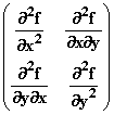
Notice that if we make a matrix out of the four possible partial derivatives (two choices for first, with respect to x or y, and then the same two choices for second derivative) in the obvious way

(The determinant of this matrix is the discriminant, of the quadratic, namely 4ac - b2.)
How does such a quadratic behave?
If a and c are both positive while b is 0, behavior in each variable here looks like that of x2 in one dimension and f will have a minimum at (x0, y0).
If we reverse all signs making a and c negative, again with b = 0, the quadratic will have a maximum at this point just as -x2 - y2 has at (0, 0).
But now there is a third possibility, that of a saddle point.
A saddle point is a critical point at which the function rises in some directions and falls in others.
There are two examples that illustrate it: x2 - y2 at (0, 0); and xy at (0, 0).
The first of these increases if you move away from the origin in directions for which |x| > |y| and not otherwise.
The second increases when both variables have the same sign, and not otherwise.
It is also possible to have behavior in which the function increases (say) in some directions and is flat in another: like x2 in two dimensions. I don't know what you should call that behavior. As in one dimension, when this happens you have to look to higher derivatives in the derivative = 0 direction to know whether you have a true local maximum or minimum.
Exercise 11.1 Find a critical point of (x - y - 1)xy. What kind of behavior does it have at that point? (You can test in an applet.)
In the applet here you can enter functions with saddle points. The origin of the name then becomes clear.
|
|