20.109 | Fall 2007 | Undergraduate

Laboratory Fundamentals in Biological Engineering

Labs

Lab work is divided into three modules. This page presents details only for the first two modules. Details of the third module are not available in OpenCourseWare, because the module is based on recent research that is being prepared for formal publication.

For modules 1 and 2, each lab session is presented on a linked web page with an introduction, protocol, and reagents list, followed by a “for next time” homework assignment.

Lab Basics

General Lab Policy

  • General dos and don’ts of working in the lab.

Guidelines for Maintaining Your Lab Notebook

  • How to maintain a good lab notebook.

Guidelines for Working in the Tissue Culture Facility

  • Procedures for doing tissue culture work.

Orientation Session (First Class)

Lecturer: Dr. Natalie Kuldell

There are six stations for you and your lab partner to visit on this lab tour. Some will be guided tours with a TA or faculty there to help you and others are self-guided, leaving you and your partner to try things on your own. Your visit to each station will last 10-15 minutes. It doesn’t matter which station you visit first but you must visit them all before you leave today. Your lab practical next time will assess your mastery of each station.

Day 1: Lab Tour

Module 1: Genome Engineering

Instructors: Prof. Drew Endy, Dr. Natalie Kuldell, and Dr. Agi Stachowiak   
Lecturer: Prof. Drew Endy   
TA: Laure-Anne Ventouras

In this experiment, we will consider the genome of a virus, namely the bacteriophage M13. M13 is a self-assembling nano-machine with a compact genome that has been optimized by evolution to commandeer its bacterial host. Approximately 1000 new viruses are generated from a single infection event. Imagine harnessing this production. What could we build and what natural processes could we better understand? One approach we’ll take is to modify the existing genome in a subtle but useful way, namely by adding a useful sequence-tag that modifies the bacteriophage coat. We’ll examine how this modification affects the coat protein’s expression and overall phage production. Another approach we’ll take is to start from scratch, undertaking a full throttle redesign of the bacteriophage genome. We’ll employ a commercial DNA synthesis company to compile the redesigned genomic program and then we’ll see if it encoded infective M13 and if the genome of the bacterial host affects bacteriophage production. Through these investigations we’ll ask: is nature’s M13 genome “perfect” or can we do better?

Photo of M13-coated coli removed due to copyright restrictions.

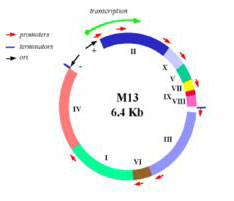
Map of M13 genome from M. Blaber. (Images courtesy of Dr. Michael Blaber. Used with permission.)

MODULES DAY LAB TOPICS
1 Start-up genome engineering
2 Agarose gel electrophoresis
3 DNA ligation and bacterial transformation
4 Examine candidate clones
5 M13.1
6 Western analysis
7

Probe western

Lecture on environmental health and safety (no materials)

8 Oral presentations

Working Page for M13 Refactoring

Pedagogy

TA’s Notes for Module 1

Module 2: Expression Engineering

Instructors: Dr. Natalie Kuldell and Dr. Agi Stachowiak   
Lecturer: Dr. Natalie Kuldell   
TA: Alice Lo

In this experiment, we will consider unintended and unpredicted effects of an experimental perturbation. Our goal is a precise one, namely to silence gene expression of a measurable gene, luciferase, using RNA interference (RNAi). Each group will begin by designing a short interfering RNA (siRNA) against luciferase, but as we’ll see, siRNAs can vary in efficacy and specificity. After transfecting a mammalian cell line with the siRNA you’ve designed and a reporter plasmid, we will evaluate the silencing using a luciferase assay and microarray technology. The first assay evaluates the efficacy of the siRNA in silencing. The second assay gives genome-wide expression data to reveal the specificity of your siRNA for the gene you’ve targeted. Through this combined approach, we’ll assess the balance of targeted and off-target effects.

Child jumping through sprinkler, with sunlight. Photo by Natalie Kuldell.

MODULES DAY LAB TOPICS
1 siRNA design and introduction to cell culture
2 Transfection
3 Luciferase assays and RNA prep
4 Journal article discussion
5 cDNA synthesis and microarray
6 Microarray data analysis
7 High throughput technologies (no materials)
8 Oral presentations

Pedagogy

TA’s Notes for Module 2

Module 3: Biomaterials Engineering

“Invention” is a wonderful word, derived from words meaning “scheme” and “a finding out.” Inventors draw on materials provided by the natural world, refining and combining them in insightful ways, to make something useful. In this experimental module we will invent materials by manipulating biological systems, namely the bacteriophage M13. We will use a very slightly modified phage to build Iridium nanowires that we’ll visualize on the transmission electron microscope. Then we’ll let the phage themselves do the building, making an electrochromic device that’s both fun and potentially useful. Drawing on the rich stockroom of biological elements and a good but incomplete understanding of their behavior, we’ll hope to invent some novel materials with real-world applications.

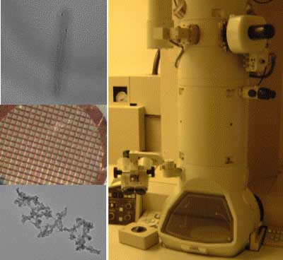
TEM of M13E4 after CoCl2/NaBH4 treatment, image courtesy of Natalie Kuldell, Anthony Garratt-Reed and KiTae Nam.

Details of this module are not available in OCW, because the module is based on recent research that is on the way to formal publication.

Lab Attendance

Lab attendance is mandatory and there are no make-up labs. A family crisis or severe illness requiring attention from the infirmary and prohibiting you from all your coursework are acceptable reasons for missing lab and every effort will be made to accommodate you in these exceptional circumstances.

Things to Do

  1. Be on time. At the start of the lab period, there will be a short introduction to the experiment you will perform that day. It is unfair to your partner and to others in the lab if you are not up to speed when the work begins.
  2. Inform the instructor and/or TA if there is a problem. You will have their immediate attention if you have cut yourself (even if you consider it minor), if something broke and needs cleaning up, or if you are on fire.
  3. Be aware of all the safety devices. Even though the instructor and TA will take care of emergencies, you should know where to find the first aid kit, the chemical spill kit, the eye wash and the safety shower.
  4. Keep clutter to a minimum. There is a coat rack to hang your jackets and there are empty cabinets to store your backpacks. Anything left in the aisles is likely to be stepped on and is a hazard to everyone.
  5. Wash your hands before you leave the lab for the day.
  6. Be aware of others in the lab. Areas of the room may be crowded at times and you should take care not to disturb the experiments of others in the lab.
  7. Bring your lab notebook and an open mind to every lab meeting.

Things Not to Do

  1. Do not eat, drink, chew gum, smoke or apply cosmetics in the lab. Just being in lab makes your hands dirtier than you can imagine and you don’t want to accidentally eat any reagent (see item 5 on ’things to do’ list).
  2. Do not put pieces of lab equipment in your mouth. It sounds obvious but you’d be surprised!
  3. Do not work with chemicals until you are sure of their safe handling. This includes some awareness of their flammability, reactivity, toxicity, and disposal.
  4. Do not use the phone or computer with gloves on your hands.

Lab notebooks are kept to document and organize your experimental plans and data. Every lab requires each researcher to keep one. Yet no two scientists organize their lab notebooks identically, and there isn’t one “right” way for you to keep yours. There are some common elements that all lab notebooks share and some important habits you should develop in keeping your notebook for this class. All lab notebooks should be…

1. Complete

Your notebook is a place to collect descriptions of experimental goals, experimental procedures, all the data you collect, and your interpretations of results. Numerical data and calculations should be written directly into your notebook, not on scraps of paper to be entered later. Data in the form of a photo should be taped into your notebook. Printouts and X-ray films can also be taped into your notebook or if reams of paper and large films are being collected, they can be organized in a separate binder and referenced in your notebook.

2. Organized

Some scientists arrange their notebooks by date, others by the question being tested. What works best depends on the research itself and the researcher. Since this class has four experimental modules that are performed sequentially, your notebook will, by default, be organized by both date and project. You will keep a record of every lab meeting, including both the date and the module/day in your notebook.

3. Up to Date

For this class, that means coming to lab with the date, module/day, title, purpose, and description already entered in your notebook. It will occasionally be helpful to have data tables ready or some calculations performed as well. “Up to date” also means leaving lab with your protocol and any amendments you made to it, data, and perhaps some interpretation entered in your notebooks. Your notebook does not need a table of contents, but you should realize that most research notebooks do.

4. Permanent

Use pen when you write in your notebooks.

Some Other Things You Should Know About Lab Notebooks

  • They are the property of the research lab itself. Researchers who join the lab after you have left it will get to know you through the notebooks you have kept there. Ideally, your notebooks will reflect your most organized, clear and thoughtful side.
  • They are legal documents. Labs in industry have special rules about lab notebooks since patent disputes and court cases often hinge on lab notebook entries.
  • They are both personal and public. It is considered impolite and an invasion of privacy to read someone else’s notebook without their permission. Most people are happy to show you their notebooks when asked.

Evaluation

Grading your Notebook

Teaching assistants will collect the duplicate copy of your notebook pages and evaluate them as follows:

LAB NOTEBOOK EVALUATION
Date of experiment √- √+
Module/Day # √- √+
Title for experiment √- √+
Brief statement of purpose √- √+
Protocol √- √+
Tables for data entry √- √+
Calculations entered √- √+
Data labeled √- √+
Summary/Interpretation √- √+
Overall √- √+

Things to Remember

Remember the goal of your notebook is to help you repeat your experiments with the same results. Information you should record includes:

  • Centrifuge settings: temperature, speed, time
  • Incubator settings: temperature, time, and shaking speed if applicable
  • Size and types of tubes used
  • Buffers (and their pH)
  • Media
  • Dilutions and how they were prepared
  • Concentrations
  • Volumes used
  • Washes: number, volumes, temperature, solutions used
  • Antibody: dilutions, lot or tube #s
  • Electrophoresis: agarose or acrylamide percentages, voltages, times
  • The names of people who helped you with your experiment

You should also note any changes to the protocol such as:

  • unexpected delays (“waterbath wasn’t ready so tubes kept on ice for one hour”)
  • unanticipated conditions (“roller drum found off in AM”)
  • unusual observations (“a large number of cells seemed to be floating”).

Good cell culture technique will simultaneously protect you from anything dangerous that might be living with the cells and protect the cells from contamination by you. You will be working with an established cell line unlikely to carry any agents that could harm you. Consequently, the guidelines here emphasize techniques for maintaining healthy and uncontaminated cells. Some points are particular to the 20.109 cell culture facility but most are common practice and will be good habits for any tissue culture work you do.

Maintaining Cultured Cells

Feeding

As cells grow and divide in a dish, they use up the nutrients provided by the media. Old media must be removed and the cells must be “fed” with some fresh media. This must be done every two or three days for most animal cell lines.

Splitting

Cells growing in a dish begin to crowd each other and then stop growing. This crowded state is called “confluence” and to maintain cells, confluent cultures must be “split” and “reseeded” into new culture dishes at a lower density.

Freezing

Every lab that works with cultured cells has a freezer stock of each cell line they study. The freezer stock is a critically important resource for the lab, storing lines that aren’t in use but are worth saving and also providing “back-up” cells if working cultures get contaminated.

Hood Preparation

  1. Wear gloves to protect yourself but also to prevent dry skin and micro-organisms from contaminating your samples.
  2. Swab down the work surface liberally with 70% ethanol. Start from the back and proceed forward. Swab during work if necessary.
  3. Swab any instruments that will be used in the hood with 70% ethanol, particularly the pipettes, which will often be used above biological samples.
  4. Keep sterile pipette tips in “Hood Only” boxes that are opened only in a sterile environment. Swab the exterior of the box with 70% ethanol.
  5. Bottles should always be tightly capped when outside the hood (i.e., they should have been tightly capped the last time they were in the hood).
  6. Dry bottles thoroughly if they have been taken out of the water incubator. Swab them with 70% ethanol, especially at the neck and the bottom, and place them directly into the hood. Avoid shaking them vigorously during handling.
  7. Bring only the items you need for a particular procedure into the hood to prevent cluttering your working space. Having a clear working space will significantly reduce the chance of contamination! Ensure easy access to items in the hood and maintain plenty of clear space in the center of the hood to work in.

Sterile Handling

  1. Spray gloves with 70% ethanol as often as necessary.
  2. The indicator stripes on the autoclave tape should turn black if an object has been properly autoclaved.
  3. Never block the negative pressure zone (also the frontal non-sterile area) of the vertical laminar flow hood with objects (i.e., notebooks, pipetteman handle).
  4. Avoid working too close to the front of the hood. Keep working area at the center or towards the back. Keep the objects needed for the current procedure within reach; keep the others in the back.
  5. Avoid working above an open bottle or dish in vertical laminar flow. Always work around them unless they are capped or covered.
  6. Avoid leaving bottles, dishes, and flasks open when they are not in use. If the cap must be laid down, place it face-up/face-down towards the back of the hood where there is less traffic and less chance of being touched or crossed over. Correct cap placement has been debated. Having a cap facing up can potentially introduce airborne particles and drive non-sterile lid liquid onto the interior face of the cap, where contaminations can fall into the bottle upon recapping. If face-down placement is preferred, then make sure to swab the area specifically and thoroughly before the cap is placed down there. Conversely, if hood surface sterility cannot be absolutely guaranteed due to high traffic or cluttering, then face-up is a better option. The best placement, however, is to place the cap on its side and towards the back of the hood. This way the interior is not in contact with the air flow or with the work surface. However, this is not possible with dishes. Therefore, exercise good judgment in light of individual operating style and the hood setup.
  7. Never pour from one sterile container to another. Pouring will generate a liquid path to introduce infection from the outside to the inside. Always pipette or use filters when transferring from one bottle to another.
  8. Mop up any spills immediately and swab with 70% ethanol to prevent the growth of microorganisms.
  9. Withdraw a pipette from its wrapper at the center of the work area, tilt it so the tip (bottom end) is pointing away from the frontal non-sterile area and away from other objects in the hood.
  10. Withdraw the pipette so that it slides through the sterile interior of the wrapper without touching the outside of the wrapper.
  11. Avoid contact between the tip of the pipette and the mouth of the bottle. The mouth and neck of the bottle (both inside and out) present a potential source of contamination.
  12. When working with Pasteur pipettes, do not reach into the box to remove it. Instead, shake the box gently to cause the pipettes to slide out slightly, and then withdraw a pipette without touching the other pipettes or the tube interior.
  13. To keep the hood from being cluttered, do not leave any trash in the hood. Immediately discard uncontaminated wrappers in the regular trash. Put all pipette tips and biologically contaminated sharps in the sharps biohazard waste container. Put all biologically contaminated tissue culture plates, flasks, and other non-sharps in the non-sharps biohazard waste container. However, an effort to minimize entry/exit from the hood should be made to minimize disturbances in the laminar flow at the entrance, which may create the potential to waft in contaminants.
  14. Handle the pipette with a steady hand. Avoid large motions and do not let the tip touch anything non-sterile. Keep the tip away from the front and far above the objects in the hood.
  15. Do not fill a dish/flask so full or swirl it such that the medium spills over the edge. This will introduce a path of infection via liquid and may cause cross-contamination.

Cleaning Up

  1. Cap bottles tightly before removing them from the hood.
  2. Swap down the work surface liberally with 70% ethanol.
  3. Turn off the vacuum, if used.

There are six stations for you and your lab partner to visit on your lab tour today. Some will be guided tours with a TA or faculty there to help you and others are self-guided, leaving you and your partner to try things on your own. Your visit to each station will last 10-15 minutes. It doesn’t matter which station you visit first but you must visit them all before you leave today. Your lab practical next time will assess your mastery of each station.

Contents

  1. Introduction to pipetting
  2. Introduction to our microscopes
  3. Introduction to our “back room” and tissue culture facility
  4. Introduction to making solutions
  5. Introduction to our spectrophotometer
  6. Introduction to lab math
  7. For next time

Introduction to Pipetting (Guided)

Someone will show you how to use your pipetmen and then you will use them to dilute a blue dye (0.01% Xylene Cyanol).

  1. If you have never used pipetmen then you should practice by pipeting 800, 80 and 8 µl of the 0.01% XC stock into eppendorf tubes. XC is not hazardous but it will stain your clothes. Pipet each volume three times and visually inspect how well the volumes match.
  2. Using your P20, measure 10, 15 and 20 µl of the 0.01% XC stock solution into the bottom of three cuvettes. Using your P1000, add water to bring the final volume to 1 ml (=1000 µl).
  3. Using your P200, measure 20, 50 and 100 µl of the 0.01% XC stock solution into the bottom of three more cuvettes. Using your P1000, add water to bring the final volume to 1 ml.
  4. Using your P1000, measure 100, 200, and 400 µl of 0.01% XC solution into the bottom of three more cuvettes. Add water to bring the final volume to 1 ml.
  5. With a gloved hand or with a piece of parafilm over the lip of the cuvette, invert each cuvette several times to thoroughly mix the contents.
  6. Visually compare your dilutions to the reference ones. If time permits, you will read the absorbance of your dilutions in the spectrophotometer so do not throw them away.

Introduction to Our Microscopes (Guided)

Much of biology examines natural components that are too small to see. Imaging technology took a gigantic step forward in the 1680s when Anton van Leeuwenhoek ground a microscope lens sufficiently fine to see a living cell (a bacteria he had scraped from his teeth!). His microscope had one lens and the image he saw was approximately 250 times its natural size (250X magnification). Compound microscopes, like the ones we have in lab, use a second lens to magnify the image from the first and can increase the total magnification up to 1000X. One of our microscopes is also attached to a beam splitter that allows excitation light to be separated from emitted light. This allows us to perform fluorescence microscopy.

No matter how fine its lens, a light microscope cannot distinguish objects closer than 200 nm. The resolution of light microscopes is limited by both the wavelength of white light (300-700 nm) and the scattering of light by the object it strikes. For better resolution, great lenses must be combined with shorter wavelengths, such as those followed by electrons or lasers, and better ways of focusing the beam such as forcing it to travel through a vacuum or an oil. Linking the microscope to a computer with digital image processing can also enhance its images. The sample itself can also be stained or fluorescently tagged to improve detection of its features.

Conventional microscope.

Fluorescent microscope.

Today you will be shown how to use each of the microscopes in the main lab and you will use them to examine some different cell types. You will be asked to focus a sample during the lab practical next time.

Introduction to Our “Back Room” and Tissue Culture Facility (Guided)

Our lab is beautifully equipped. We have a fume hood for work that generates hazardous vapors. We have a back room where dishes can be washed and material can be decontaminated. The backroom also has an icemaker, a sink with ultrapure water and several CO2 tanks that feed into the incubators in the tissue culture facility.

The tissue culture facility has three hoods with germicidal lamps, six incubators for growing eukaryotic cells, two inverted microscopes, and a tabletop centrifuge. It also has a waterbath for warming up solutions and a refrigerator for keeping them cool.

Today you will be shown how to use the autoclave and what it does. You will also be shown some key features of the tissue culture facility, including the different types of waste disposal containers (for trash, biohazard, sharps). More formal training in tissue culture techniques will occur as part of experimental module 2.

Introduction to Making Solutions (Self-Guided)

Today you will make 100 ml of a 0.5M sorbitol solution and measure its pH. Making solutions is a fundamental part of being in lab and the success of your experiments is absolutely dependent on doing it correctly and consistently. If you are unclear about any of the following instructions, be sure to ask for help.

Balance.

pH meter.

Part 1: At the Balance

  1. Put on gloves to weigh out solids. This protects you from the chemicals and the chemicals from getting contaminated with anything foreign on your hands. Sorbitol is not a dangerous chemical.
  2. Zero the balance with a medium size weigh boat on it. Weigh boats are kept in the drawer under the balance. The marked → O/T ← will zero (“tare”) the balance and the display should read 0.0000 after taring. Be sure to close the balance doors when taring the balance.
  3. Use a spatula to measure 9.1 grams of sorbitol. To measure this, open the balance doors and hold the spatula and chemical over the weigh boat. Begin by adding only a small amount of the powder to the weigh boat. Once you determine how much that weighs, you can add correspondingly more. If you have weighed out too much, you can put some back as long as you have used a clean spatula and a clean weigh boat.
  4. Remove the weigh boat with your sorbitol from the balance, gently bend the ends together and pour the contents into a beaker. Tap the back of the weigh boat to loosen any powder that is stuck. The weigh boat can be discarded in the trash since sorbitol is not dangerous.
  5. Clean the balance with a brush. Clean the area around the balance with a wet paper towel.

Part 2: Measuring Liquids and Mixing

  1. Measure approximately 80 ml of ultrapure water into a 100 ml graduated cylinder. Read the volume in the cylinder by bringing it to eye level to see where the meniscus reaches. Add the water to the beaker with your sorbitol.
  2. Gently drop in a magnetic stir bar with a diameter approximately ½ that of the beaker. Magnetic stir bars are kept in the drawer below the balance.
  3. Put the beaker on the stir plate and turn the stirrer on slowly. The stir bar should spin fast enough to form a vortex in the center of the beaker. You do not want the stir bar to bump around in the beaker since this can break the beaker. If the stir bar is stirring unevenly, then turn off the stir plate, allow the magnetic stir bar to stop, and then start it again.
  4. Stir until all the powder is dissolved.
  5. Pour the solution back into your graduated cylinder.
  6. Add ultrapure water up to 100 ml using a plastic disposable pipet. To open the pipet, hold it in one hand. With the other hand puncture the wrapper by pulling it against the top of the pipet (not the end with the tip!). Put the exposed end of the pipet into the pipet aid or bulb then withdraw the pipet from the rest of the wrapper. Place the tip of the pipet into the ultrapure water and withdraw enough water to “top off” your solution. Dispense the water into your sorbitol by submerging the tip of the pipet into the solution and releasing the water from the pipet. Stop when the graduated cylinder reads 100 ml. Extra water can be discarded into the sink and the used pipet can be discarded in the sharps waste container that is under the bench.

Part 3: Measuring pH

  1. Since you will measure the pH of your solution you should pour it back into your beaker and put it on a stir plate. Start the stir bar gently spinning. If you did not have to measure its pH you would move it to a bottle for storage.
  2. Remove the pH electrode from the storage solution and rinse it over the waste beaker using distilled water from the wash bottle. A Kimwipe can be used to gently dry the electrode.
  3. Place the electrode ½ way into the 15 ml conical tube with calibration buffer pH 7.0. Press the “read” button. Wait for the reading to stabilize and note how close it is to pH 7. Press the “read” button again to put the pH meter on standby.
  4. Rinse and dry the electrode then place it in your sorbitol solution. Hold the electrode at the edge of the beaker and be careful not to let the stir bar hit (and break!) the electrode. Read the pH of your solution and let one of the teaching faculty know what you have found.
  5. Rinse and dry the electrode then return it to the electrode storage solution.
  6. Pour the sorbitol solution (but not the stir bar!) down the sink. Rinse the beaker with tap water and return it to the balance area. Dry the stir bar and return it to the drawer.

Introduction to Our Spectrophotometer (Self-Guided)

Color is created when a white light strikes a molecule that then reflects light of a certain wavelength and absorbs all the others. A spectrophotometer is an instrument that measures the amount of light absorbed by a sample. It does this by shining light of a particular wavelength into a sample and measuring how much light comes all the way through. Samples are held in cuvettes between the light source and the detector.

Measuring absorbance. (Figure by MIT OpenCourseWare.)

Here are two important things to remember about spectrophotometers. First, different compounds absorb different wavelengths of light. Red pigments absorb blue light (light of ~300 nm wavelengths) and blue pigments absorb red light (light of ~600 nm wavelengths). Therefore all spectrophotometers have ways of adjusting the wavelength of light shining into the sample. The second important point is that the amount of light absorbed by a sample is directly proportional the concentration of that sample. This is a very useful relationship, making the spectrophotometer a valuable research tool.

Spectrophotometer.

Cuvette holder.

Part 1: Using the Spectrophotometer

In this assay you will calibrate your pipets by measuring the absorbance of the XC dilutions you made. Beer’s Law, which relates absorbance to concentration, will be derived as part of experimental module 2. Here, you’ll see that the graph of absorbance versus volume of 0.01% XC is a straight line… or at least it should be!

  1. Using your P1000, measure 1 ml of water into a plastic cuvette. This cuvette will serve as your blank for the spectrophotometer.
  2. Confirm that the machine is set to read absorbances at 600 nm.
  3. Put your blank into the spectrophotometer at position 1, which is furthest back in the instrument. Be sure the window of the cuvette and not the frosty sides are in the light beam that travels from left to right.
  4. Close the door of the spectrophotometer. Click “blank” (lower left of the screen). A “reading blank” message should appear. When the message is gone, then the blank is set.
  5. Replace the blank with your first sample. Close the door of the spectrophotometer. Click “read samples” (upper left of the screen). Write down this value.
  6. Repeat with all your samples.
  7. Remove your last sample. Close the door of the spectrophotometer.
  8. The XC dilutions can be washed down the sink and the cuvettes can be discarded in the sharps bin.

Part 2: Considering your Data

  1. Use Excel to prepare a graph of absorbance versus volume of 0.01% XC. Some sample graphs are reproduced below and you should generate similar ones with your data. Be sure to include a trendline, displaying its equation as well as the r-squared value on the graph. The r-squared value reflects how well the data points fit the equation. A perfect fit will give an r-squared value of 1. If you are uncertain how to make such a graph using Excel, be sure to ask for help. We will use Excel a lot this semester, in particular during experimental module 2.
  2. If the pipets were well calibrated and the measurements were done carefully, then the points should fall close to a straight line, and the r-squared will be close to 1. If one point seems way off, you can repeat the three measurements for that pipetman. If the second set of data does not look linear, we can clean the inner workings of your pipetman before you try the assay again.
  3. There should also be good agreement between the 20 µl measurements made with the P20 and the P200 as well as the 100 µl measurements made with the P200 and P1000. Is there?

Left to right: P20 calibration, P200 calibration, and P1000 calibration.

Introduction to Lab Math (Self-Guided)

The information and exercises provided here are intended to refresh your memory of these concepts. If they are entirely new to you or if you are struggling with the practice problems, please ask for extra help. It is absolutely essential that you are comfortable with the information presented here.

Part 1: Metric System

This is the numerical language of science. Base units that you will most often use in this class are meters, grams, liters, and moles. These units will be appended with prefixes to modify the unit by a power of ten.

103  = 1000     = 1000/1    = 103/1   kilo (k-) 100  = 1        = 1/1       = 100 /1  base unit (-g, -l, -mole…) 10-3 = 0.001    = 1/1000    = 1/103   milli (m-) 10-6 = 0.000001 = 1/1000000 = 1/106   micro (µ-)

Practice problems:

  1. The distance between two cells in 800 µm. How many mm is that?
  2. The amount of sorbitol you want to weigh is 1.9 g. How many mg is that?
  3. The volume you want to measure is 100 ml. How many liters is that?
  4. Your reaction generates 0.1 µmoles of product. How many mmoles is that?

Scientific notation expresses numbers so there is one digit to the left of the decimal point and that number is multiplied by a power of ten. 2334 becomes 2.334 x 10³ and 0.0041 becomes 4.1 x 10⁻³. Computations are easier with numbers in scientific notation and some numbers that are easier to write (602,214,199,000,000,000,000,000 versus 6.02 x 10²³).

Practice problems:

Convert the following to scientific notation

  1. 1000
  2. 2
  3. 0.0023
  4. 0.000000467

The metric system and scientific notation go hand in hand, making unit conversions straightforward. For example 100 µl can be converted to ml by writing the starting volume in scientific notation (1.00 x 10² µl) and multiplying by the power of ten that separates the units (1 ml = 1 x 10³ µl). Set up every equation so the units will cancel properly when you multiply through.

Practice problems:

Be sure you can express your answers in scientific notation.

  1. How many ml is 100 µl?
  2. How many mg is .023 g?
  3. How many mmoles is 250 µmoles?

Part 2: Concentrations

Molarity (moles/liter) is a common expression of concentration. When making a solution of a particular molarity, you need to know three things: the desired molarity, the desired volume and the formula weight of the compound to be dissolved. The best place to find the formula weight (grams/mole) is on the chemical’s bottle. Calculations are performed by setting up an equation so that the units cancel, leaving grams in the numerator and volume in the denominator.

Another common expression of concentration is percent. Percent solutions are always based on 100 ml. For powdered substances, percent solutions reflect the weight in a 100 ml volume (“w/v”). For example a 10% solution of NaCl is 10 grams in 100 ml of water. In fact a 10% solution of any powdery substance is 10 grams in 100 ml. For liquids, percent solutions reflect the volume in a 100 ml final volume (“v/v”). For example a 70% ethanol solution is 70 ml of 100% ethanol and 30 ml of water. Remembering that 1 ml of water weighs 1 gram may help you remember the w/v and v/v expressions.

Practice problems:

  1. You want to make 100 ml of a 0.5M sorbitol solution. The formula weight of the substance you want to dissolve is 182. How many grams will you measure?
  2. You want to make 10 ml of a 0.01% (w/v) solution of XC. How many grams will you dissolve?
  3. How would you make 100 ml of a solution that is 5% (v/v) acetic acid and 5% methanol?

Part 3: Dilutions

Many solutions are made by diluting concentrated stock solutions. Dilution factors of 1:2, 1:5, 1:10 and 1:100 are common. These dilutions are made by diluting one “part” stock with 1, 4, 9 or 99 “parts” water. For example, you could make 100 ml of a 0.5M sorbitol solution by mixing 10 ml of a 5M stock solution with 90 ml of water. This is a 1:10 dilution of the stock. The dilution factor can be converted to a fraction to determine the solution’s final concentration (5M x 1/10 = 0.5M).

When the dilution factor is less obvious, the formula C1V1 = C2V2 can be used, where C1 is the starting concentration of the stock solution, C2 is the desired concentration, V1 is the volume of stock you’ll need (usually this is your unknown) and V2 is the final volume you want to make. For example, to make 1000 ml of a 0.2M Tris from a 1.5M stock you would multiply 1.5M (V1) = 0.2M (1000) to find that you will need 133 ml of the stock. To determine how much water to add you would subtract V2 – V 1, in this case 1000 ml –133 ml = 867 ml of water.

When solutions must be diluted several orders of magnitude, then serial dilutions are made. The concentrated stock is progressively diluted, for example using a 1:100 dilution as the new “stock” in another 1:100 dilution. Such a serial dilution produces a solution that is 10,000 times less concentrated than the starting material. One benefit to serial dilutions is that small volumes of each dilution can be made accurately. A drawback is that any pipetting or calculation error is propagated through every dilution.

Practice Problems

  1. How would you make 50 ml of a 1:5 dilution?
  2. Give the volume of stock and the volume of water necessary to make 50 ml of a 0.25 M solution starting with a 2M solution.
  3. A concentrated culture of bacteria has approximately 1 x 10⁸ cells/ml. What is the concentration of bacteria after it has been diluted 1:100? What is the concentration of bacteria if a 1:2 dilution was made of the 1:100?

DONE!

For Next Time

  1. Review today’s lab to prepare for the lab practical that you and your partner will take together.
  2. Complete the required EHS Training on-line.
    • There are two Web-based training modules required for 20.109, accessed through MIT’s Environmental Health and Safety page. They are Chemical Hygiene Training and Managing Hazardous Waste. Chemical Hygiene includes 7 sections and 6 quizzes with an estimated completion time of 1 hour. The Managing Hazardous Waste training is one quiz and should take less than ½ hour to complete.
    • If you have completed EHS training in a UROP or in another lab class, you do not need to repeat the training but you do need to print out your training record to hand in.
    • From the EHS training page select the second button labeled “I have EHS training requirements for an academic subject.”
    • Your summary page (“My EHS Training”) should show Chemical Hygiene and Managing Hazardous Waste as requirements for 20.109. Click on the purple button “Go to Web Classes” right above the training requirements section. You may stop and start the Web-based courses as many times as you need to for completion. The software keeps track of where you are in the course.
    • Print the certificate of completion to turn in next time.
  3. Register for an account on OpenWetWare by filling out the “Join OWW” form. Once you get an account:
    • familiarize yourself with using the wiki by reading the “OpenWetWare Basics” page.
    • add the 20.109 home page to your “watch” list so you’ll be notified by email when an announcement is made.
    • add your user page to the class “People” page and put some information on your user page. Be careful about how you put your e-mail address on your page; make sure to spell out “at” or otherwise break your address up so it can’t be scraped up by spambots.
  4. Complete the student registration/questionnaire to turn in next time.
  5. Be prepared to Start up Genome Engineering, by reading the introduction at that link. It describes some basic information that you’ll need for the experiment that you’ll start next time. Come to class next time familiar with some of the life cycle of the M13 bacteriophage as well as a copy of its Genome Sequence.

Modules: 1.1 | 1.2 | 1.3 | 1.4 | 1.5 | 1.6 | 1.7

Introduction

How many genetically-encoded creatures exist in every milliliter of sea water? 100? 1000? More? It turns out that bacteria are by far the best represented life form, numbering up to a million cells/ml. If each cell is assumed to harbor the DNA content of pedestrian E. coli MG1655, then that means 1012th base pairs of DNA/ml. This thriving gene pool is even more remarkable in light of the fact that each ml of sea water contains approximately 1010th viruses that infect bacteria, aka bacteriophages or “phages” for short. These destroy half the world’s bacterial population every 48 hours [2]. Given the huge number of bacteriophages that exist, it’s probably not surprising that most of the Earth’s bacteriophages are completely uncharacterized, though massive genome sequencing efforts are underway.

A few bacteriophages are exquisitely well characterized. Indeed, the study of phage laid much of the groundwork for our current understanding of genetics and molecular principles in biology. These principles carry over to the biology of more complex cells (Jacques Monod famously said “What is true for Escherichia coli is true for the elephant” [Francois Jacob (1988)]). M13 is a member of the filamentous phage family. It has a long (~900 nm), narrow (~20 nm) protein coat that encases a small (~6.4 Kb) single stranded DNA genome. The genome encodes 11 proteins, five of which are exposed on the phage’s protein coat and six of which are involved in phage maturation inside its E. coli host.

Phage Particles

The phage coat is primarily assembled from a 50 amino acid protein called pVIII (or p8), which is sensibly enough encoded by gene VIII (or g8) in the phage genome. For a wild type M13 particle, it takes about ~2700 copies of p8 to make the ~900 nm long coat. The coat’s dimensions are flexible though and the number of p8 copies adjusts to accommodate the size of the single stranded genome it packages. For example, when the phage genome was mutated to reduce its number of DNA bases (from 6.4 kb to 221 bp) [3], then the p8 coat “shrink wraps” around the reduced genome, decreasing the number of p8 copies to less than 100. Electron micrographs of the resulting “microphage” and its wild type parent are shown below (image courtesy of Esther Bullitt, Boston University School of Medicine), where the black bar in each image is 50 nm long. And what about the upper limit to the length of the phage particle? Anecdotally, viable phage seems to top out at approximately twice the natural DNA content. However, deletion of a phage protein (p3) prevents full escape from the host E. coli, and phages that are 10-20X the normal length with several copies of the phage genome can be seen shedding from the E. coli host (look at the image on the coverpage to this module).

Figure 1. Electron micrographs of microphage described by Specthrie, et al. Source: Specthrie, L., et al. “Construction of a Microphage Variant of Filamentous Bacteriophage.” J Mol Biol 228, no. 3 (December 5, 1992): 720-724. Courtesy of Elsevier, Inc. ScienceDirect. Used with permission.

There are four other proteins on the phage surface, two of which have been extensively studied. At one end of the filament are five copies of the surface exposed pIX (p9) and a more buried companion protein, pVII (p7). If p8 forms the shaft of the phage, p9 and p7 form the “blunt” end that’s seen in the micrographs. These proteins are some of the smallest known (only 33 and 32 amino acids), though some additional residues can be added to the N-terminal portion of each which are then presented on the “outside” of the phage coat (much more on this technique later). At the other end of the phage particle are five copies of the surface exposed pIII (p3) and its less exposed accessory protein, pVI (p6). These form the rounded tip of the phage and are the first proteins to interact with the E. coli host during infection. p3 is also the last point of contact with the host as new phages bud from the bacterial surface.

Phage Life-cycle

The general stages to a viral life cycle are: infection, replication of the viral genome, assembly of new viral particles and then release of the progeny particles from the host. Filamentous phages use a bacterial structure known as the F pilus to infect E. coli, with the M13 p3 tip contacting the TolA protein on the bacterial pilus. The phage genome is then transferred to the cytoplasm of the bacterial cell where resident proteins convert the single stranded DNA genome to a double stranded replicative form (“RF”). This DNA then serves as a template for expression of the phage genes.

Figure 2. Cartoon of phage life cycle.

Two phage gene products play critical roles in the next stage of the phage life cycle, namely amplification of the genome. pII (aka p2) nicks the double stranded form of the genome to initiate replication of the + strand. Without p2, no replication of the phage genome can occur. Host enzymes copy the replicated + strand, resulting in more copies of double stranded phage DNA. pV (aka p5) competes with double stranded DNA formation by sequestering copies of the + stranded DNA into a protein/DNA complex destined for packaging into new phage particles. Interestingly there is one additional phage-encoded protein, pX (p10), that is important for regulating the number of double stranded genomes in the bacterial host. Without p10 no + strands can accumulate. What’s particularly interesting about p10 is that it’s identical to the C-terminal portion of p2 since the gene for p10 is within the gene for p2 and the protein arises from transcription initiation within gene 2. This makes the manipulation of p10 inextricably linked to manipulation of p2 (an engineering headache) but it also makes for a compact and efficient phage in nature.

Table 1. M13 protein functions.

Phage maturation requires the phage-encoded proteins pIV (p4), pI (p1) and its translational restart product pXI (p11). Multiple copies (on the order of 12 or 14) of p4 assemble in the outer membrane into a stable, i.e. detergent resistant, barrel-shaped structure. Similarly a handful of the p1 and p11 proteins (5 or 6 copies of each) assemble in the bacterial inner membrane, and genetic evidence suggests C-terminal portions of p1 and p11 interact with the N-terminal portion of p4 in the periplasm. Together the p1, p11, p4 complex forms channels through which mature phage are secreted from the bacterial host.

To initiate phage secretion, two of the minor phage coat proteins, p9 and p7, are thought to interact with the p5-single stranded DNA complex at a region of the DNA called the packaging sequence (aka PS). The p5 proteins covering the single stranded DNA are then replaced by p8 proteins that are embedded in the bacterial membrane and the growing phage filament is threaded through the p1, p11, p4 channel. This replacement of p5 by p8 explains the microphage data presented earlier…making very clear how the size of the phage particle is determined by the number of bases the phage packages. Once the phage DNA has been fully coated with p8, the secretion terminates by adding the p3/p6 cap, and the new phage detaches from the bacterial surface. How long does all this take? Amazingly, new M13 phage particles are secreted within 10 minutes from a newly infected host and can arise at a rate of 1000/cell within the first hour of infection. Also amazing is how the bacterial host can continue to grow and divide, allowing this process to continue indefinitely.

Protocols

As you heard about in lecture, you’ll be starting a project to study the M13 genome and in the process you’ll be learning some fundamental tools and techniques of molecular biology. One major goal we have for this module is to establish good habits for documentation of your work, in your lab notebook and on the wiki. By documenting your work according to the exercises done today, you will

  • Be better research students (in 20.109 and in any research lab you may join)
  • Be better writers since a clear record of what you’ve done will improve your data analysis
  • Be better scientists, since you’ll eventually train others to document things this way too

Today’s lab has four parts. First, you and your partner will complete the lab practical we have set up for you. Second, you and your lab partner will annotate the M13KO7 genome map, identifying trouble spots suitable for re-engineering. Next you will design a pair of oligonucleotides to modify the M13 genome, adding restriction sites to the gene encoding p3. Finally, you will begin to prepare the M13 backbone so next time you can clone the insert oligonucleotides you design today.

Part 1: Lab Practical

Good luck!

Part 2: M13KO7 Renovation

You are about to undertake an ambitious project, namely a major renovation of the M13 genome. If you’re successful, the renovated genome will be a better substrate for further engineering. It will consist of discrete, insulated elements that might, later on, be re-used, tuned and rationally modified with ease. Refining the genome won’t be easy. Nature has optimized the existing phage in response to evolutionary pressures and it will be a lot easier for you to kill it than to improve it. But we have a few powerful resources to draw from: full sequence data is available for the M13 genome and some of its close relatives; clever genetic experiments have defined the functionally relevant parts; structural data gives us a view of the phage particle and its components. Together these provide detailed, though not complete, understanding of the workings of the phage. And the beauty of this experiment is how your genome renovation, once built and tested, will feedback and add to the existing base of knowledge.

Today you will begin your renovation with a detailed evaluation of the natural existence, identifying parts of the genome crying out for re-engineering. Annotate the M13KO7 genome from the printout in the following way.

  1. Copy the sequence and the numbers associated with each line of sequence into a MSWord document.
  2. Read just the margins or font size so the lines of sequence are more easily read. Margins should be no smaller than 0.6’ and the font size should be no smaller than 12 point.
  3. Box the unique BamHI site (GGATCC) that starts at position 2220.
  4. Use the information printed at the start of your M13KO7 sequence to identify and then draw a box around the start (use a green box) and stop codons (use a red box) for genes I through XI. Codons for the standard genetic code can be found here. You can use the space between lines of code to note which landmark you’ve annotated (e.g. “p9 start”).
  5. Summarize in your notebook any instances where modification of one gene affects the sequence of another, or instances where the natural sequence is hard to understand or where a sequence feature makes some human-manipulation undo-able or particularly complex to perform.
  6. Add your names, your team color, your lab section and today’s date to the top of the document.
  7. Print out three copies of your document, one to hand in and one for your notebooks.
  8. Email the document to yourself since you will need it for later assignments.

Part 3: Digest M13KO7

Restriction endonucleases, also called restriction enzymes, cut (“digest”) DNA at specific sequences of bases. The restriction enzymes are named for the prokaryotic organism from which they were isolated. For example, the restriction endonuclease EcoRI (pronounced “echo-are-one”) was originally isolated from E. coli giving it the “Eco” part of the name. “RI” indicates the particular version on the E. coli strain (RY13) and the fact that it was the first restriction enzyme isolated from this strain.

The sequence of DNA that is bound and cleaved by an endonuclease is called the recognition sequence or restriction site. These sequences are usually four or six base pairs long and palindromic, that is, they read the same 5’ to 3’ on the top and bottom strand of DNA. For example the recognition sequence for EcoRI is shown in the figure. Other restriction enzymes, for example HaeIII, cut in the middle of the palindrome leaving no DNA overhang, called a “blunt end.”

EcoRI cuts between the G and the A on each strand of DNA, leaving a single stranded DNA overhang (also called a “sticky end”) when the strands separate. (Figure by MIT OpenCourseWare.)

One of the most useful resources for restriction enzyme information is the website from New England Biolabs. Use their search engine to retrieve information about the recognition enzymes SmaI and XmaI. Be sure you are clear on how they differ before you move on to the experiment. For example, do the enzymes have the same recognition sites? do they leave the same overhang? will they work in the same buffer? at the same temperature? These are some of the preliminary questions you’ll have to ask yourself whenever you set up a restriction digest.

Next, use the NEB Web site or the paper copy of their catalog to look up the recognition sites for the enzyme BamHI. What overhang does it leave? what buffer is recommended? what temperature does it work best at? You will perform a restriction digest with BamHI which cuts the gene for p3. Label two tubes with your team color, the name of the DNA you’ll digest, and the name of the enzyme (if used).

TO MODIFY g3 UNCUT CONTROL DIGEST
DNA 20 µl M13KO7 20 µl M13KO7
H2O To a final volume of 25 µl To a final volume of 25 µl
Buffer (as directed by NEB) 2.5 µl 10X NEB buffer 2.5 µl 10X NEB buffer
Enzyme None 0.5 µl BamHI

Note 1: For traditional reasons, the volume of enzyme is not included in the final volume of the reaction

Note 2: Assemble your reactions in the following order: water, buffer, DNA and finally enzyme.

Note 3: The restriction enzyme, BamHI, is a protein and so is subject to heat denaturation. Enzymes should be kept on ice and not placed in your room temperature eppendorf rack while you are using them…this will be true all term!

Note 4: You should always be careful about using clean pipet tips but it is especially important to be 100% certain your pipet tip is clean when you are using common stock reagents, like enzymes and buffers. Contamination of a lab’s common stock is incredibly hard to trace and results in lost time and aggravation for everyone.

You can flick the tube to mix the contents and give it a quick spin in the microfuge to bring any droplets down to the bottom of the eppendorf tube (be sure to balance your tube against another in the microfuge). Place both tubes in the 37° incubator while you design the oligonucleotides that you will clone into this digested plasmid. To anticipate a little bit of the nomenclature that will used: this digested plasmid is refered to as the “backbone” of your clone since most of the basic plasmid functions will be provided by this piece of DNA

Part 4: M13KO7 Tag

In the genome engineering module, you will be adding a short sequence of DNA into an existing restriction site in the M13KO7 genome. This modification will simultaneously destroy the natural restriction site and add two new unique ones. Recall, though, that any manipulation to the DNA can affect phage function since nearly every base of the phage genome encodes a gene (at least one!) and there are complex regulatory elements that are known to exist…plus ones we don’t know about yet. Despite the uncertainty, there are three important reasons to undertake the experiments you’re starting today. First, if you’re successful, then the modified phage genome will be a better substrate for later building projects. Second, this project will give us important new information about the phage’s tolerance for manipulation, since these changes have not been applied to the phage genome before. Third, you may discover new things about how that M13KO7 phage genome is organized and operates.

As you design your DNA insert, remember that there is no single “right” design. You will have a framework to operate in. This framework is occasionally constrained by practical considerations, for example we don’t have every known restriction enzyme in the teaching lab and we don’t have limitless time to work on this project. More often, though, the solution to your design task is constrained by nature, who requires triplet codons and palindromic enzyme recognition sites. So be prepared to sketch, refine, redesign and then choose your favorite experimental plan. We expect six groups will find six different solutions

Igonucleotide Design

Begin by opening and printing the translated M13KO7 g3p (PDF)

Find the BamHI site on this sequence. It should fall across an E D P sequence about halfway through the protein translation. At the bottom of the printout, write the double stranded sequence for this region, grouping the E D P sequence into the correct codon triplets and indicating the overhanging single stranded sequences you will have once the DNA is digested. Write each strand with the overhangs in lowercase letters and the other (“annealed”) bases in the traditional uppercase throughout. Now you’re ready to plan your insert. Plan the top strand of the insert first

Top Strand, Step 1

Open a new Microsoft® Word file to document your design. For each step, note the step number, the purpose, and then the sequence, including an indication of the 5’ end. Begin your top strand oligonucleotide with the 4 base overhang (in lowercase) that could anneal to the M13KO7 backbone you’ve digested with BamHI. Put a comma, slash or space between codons.

Top Strand, Step 2

If the next base in your oligonucleotide was “C” then it would regenerate the BamHI site when added back to the M13KO7 plasmid backbone. This is not desirable, for reasons that will be clear later. So pick some other base for the next base of your oligonucleotide.

Top Strand, Step 3

Add the first of two new restriction sites that will be unique to M13KO7. Review the list of zero cutter enzymes <**link to mod1.1_zerocutters.txt> that don’t cut M13KO7 can be found here. Using the base from step 2 as the first base of the new site, fill in the rest of the sequence for a new restriction site, including commas, slashes or spaces between codons. Underline the new site and then, just below the sequence, write the name of the enzyme that recognizes it.

Top Strand, Step 4

Use the 3’ base from the site designed in step 3 to add another unique site downstream. Consult the list of zero cutters **link to mod1.1_zerocutters.txt again. If the site you added in step 3 was a blunt cutter, then add a sequence with an overhang. If you’ve already added a restriction site that leaves an overhang when cut, then add a blunt cutter site with this step. Once you’ve chosen a site and added the recognition sequence to the 3’ end of your growing oligo then put commas, slashes or spaces between codons. Box the new site in your MSword document and then, below the sequence, write the name of the enzyme that recognizes it.

Top Strand, Step 5

  • Now for some important checks and documentation:
  • Confirm that the most 3’ base is not a “G” or the oligonucleotide will regenerate the BamHI site when ligated into the M13KO7 backbone. If it is a “G” then choose a different restriction site for your design.
  • Translate the codons that you’ll be adding to the protein. You use the genetic code listed at NEB. If there is a stop codon in your oligonucleotide, then you must reconsider the choices you’ve made. If there are “difficult” amino acids that you’ll be including, for example a string of prolines, then you might reconsider your design. If there are no more changes to be made to the top strand of your oligonucleotide, then write the amino acids that will be encoded above the codons that encode them on your Microsoft® Word document.

Now you’re ready to design the bottom strand. This will be a breeze, with the only really tricky part coming at the end when you turn the sequence you’ve designed around, to list it in the 5’ to 3’ direction as convention dictates.

Bottom Strand, Step 1

You’ll be designing this oligo from the 3’ end so be sure to write that on your Microsoft® Word document before listing any bases that you’ll want to include. Then write the complementary sequence to all but the first 4 bases of your top oligo. By leaving off the first 4 bases, they will remain unpaired when the top and bottom strand anneal. Though it’s not needed for translation (you’ve done that already!), it’s helpful to put a comma, space or slash between the codons just to keep yourself in register.

Bottom Strand, Step 2

Add the 4 base overhang that could anneal to the M13KO7 backbone you’ve digested with BamHI. Be sure you’re clear which end of the oligonucleotide this should be tacked onto. Also be sure you have the correct strand of the recognition site. You might want to draw a picture if you’re puzzled. Put a comma, slash or space between codons if you find that helpful.

Bottom strand, step 3: Document the oligonucleotide pair you’ve designed by “annealing” them at the bottom of your Microsoft® Word document. This will allow you to confirm the base pairing and the single stranded overhangs. You should also indicate above the pair what amino acids you’ll expect each codon to produce and indicate below the pair which restriction enzymes you expect to cut this DNA. Print out 3 copies of your Microsoft® Word document: one for you, one for your lab partner, and one for the teaching faculty.

All that’s left now is to place the order. To do this you must:

  1. Reverse the bottom strand’s sequence so it’s written in the 5’ to 3’ direction.
  2. Add the sequences to the table on the “talk” page associated with today’s lab. Note the restriction enzymes you’ll need there as well, and upload the Microsoft® Word document to keep a record of your work.

Before you leave, give your digested DNA samples to the teaching faculty, who will freeze them away for next time.

DONE!

For Next Time

All “for next time” assignments should be printed out and handed in at the beginning of the next lab period, unless otherwise indicated.

  1. The major writing assignment for this module will be a description of your M13 renovation work. Use the summary in your lab notebook to start a table on your wiki user page to organize your thoughts about the existing genome. Generate a table that lists each gene and any re-engineering ideas you have for it. Print out this table to hand in next time. If you want to start a new wiki page for this part of the assignment, go for it but be sure to follow OWW page naming guidelines and choose something like “username:superM13” as the title for your page not just “myM13” since there will soon be several people trying to name their page exactly that.
  2. Nature often preserves functionally critical genomic elements, and evolutionary cousins can help us identify which genetic elements are disposable, which are interchangeable, and which are essential. Who are M13’s closest evolutionary relatives and how do they differ from the phage you’re working with?
  3. Register for an account at the Registry for Standard Biological Parts. This site is a clearing house for engineered biological parts that can be used as substrates for building. Look up part BBa_M1307 and write a response to the following criticism: “BBa_M1307 is not a standard biological part and does not belong in the registry.”

Reagents List

1. “10X NEBuffer 1:

  • 100 mM Bis Tris Propane-HCl
  • 100 mM MgCl2
  • 10 mM DTT

2. “10X NEBuffer 2:

  • 500 mM NaCl
  • 100 mM Tris-HCl
  • 100 mM MgCl2
  • 10 mM DTT

3. “10X NEBuffer 3:

  • 1 M NaCl
  • 500 mM Tris-HCl
  • 100 mM MgCl2
  • 10 mM DTT

4. “10X NEBuffer 4:

  • 200 mM Tris-acetate
  • 100 mM MgAc
  • 500 mM KAc
  • 10 mM DTT

Modules: 1.1 | 1.2 | 1.3 | 1.4 | 1.5 | 1.6 | 1.7

Introduction

Electrophoresis is a technique that separates large molecules by size using an applied electrical field and a sieving matrix. DNA, RNA and proteins are the molecules most often studied with this technique; agarose and acrylamide gels are the two most common sieves. The molecules to be separated enter the matrix through a well at one end and are pulled through the matrix when a current is applied across it. The larger molecules get entwined in the matrix and retarded; the smaller molecules wind through the matrix more easily and travel further from the well. Molecules of the same size and charge migrate the same distance from the well and collect into a band.

DNA and RNA are negatively charged molecules due to their phosphate backbone, and they naturally travel toward the positive charge at the far end of the gel. They are typically examined with agarose gels. Proteins are composed of amino acids that can be positively, negatively or uncharged. To give proteins a uniformly negative charge, they are coated with a detergent, SDS, prior to running them on a gel. Protein samples are also boiled to remove any secondary structure that might make two molecules of the same size migrate differently. Polyacrylamide is the matrix commonly used to separate proteins. These gels are typically run vertically while agarose gels are run horizontally but gravity has nothing to do with the separation.

Diagram of agarose gel setup, for agarose gel electrophoresis. (Figure by MIT OpenCourseWare.)

Today you will separate DNA fragments using an agarose matrix. Agarose is a polymer that comes from seaweed and if you’ve ever made Jell-O™, then you already have all the skills for pouring an agarose gel. To prepare these gels, agarose and buffer are microwaved until the agarose is melted. The molten agar is then poured into a horizontal casting tray, and a comb is added. Once the agar has solidified, the comb is removed, leaving wells into which the DNA sample can be loaded.

The distance a DNA fragment travels is inversely proportional to its length. Over time fragments of similar length accumulate into “bands” in the gel. Higher concentrations of agarose can be used to resolve smaller DNA fragments. This figure shows the same DNA fragments resolved with three agarose concentrations. The 1000 base pair fragment is indicated in each.

DNA fragments resolved with three agarose concentrations. The line indicates the 1000 base pair fragment. (Figure by MIT OpenCourseWare.)

Size vs. migration distance.

Ethidium Bromide is a fluorescent dye that is commonly added to agarose gels. This dye intercalates between the bases of DNA, allowing DNA fragments to be located in the gel under UV light and photographed. The intensity of the band reflects the concentration of molecules that size, although there are upper and lower limits to the sensitivity of dyes. Because of its interaction with DNA, ethidium bromide is a powerful mutagen and will interact with the DNA in your body just as it does with any DNA on a gel. You should always handle all gels and gel equipment with gloves. Agarose gels with Ethidium Bromide must be disposed as hazardous waste in the labelled container in the fume hood.

Today you will run your M13KO7 digested samples on an agarose gel, cut the linearized backbone out of your gel and then purify the DNA from the agarose. Next time you will mix the backbone and insert in a ligation reaction.

Protocols

Part 1: Running your gel

  1. Add 2.5 µl loading dye to M13KO7 samples from last time. Loading dye contains xylene cyanol as a tracking dye to follow the progress of the electrophoresis (so you don’t run the smallest fragments off the end of your gel!) as well as glycerol to help the samples sink into the well.
  2. Flick the eppendorf tubes to mix the contents then quick spin them in the microfuge to bring the contents of the tubes to the bottom.
  3. Load the gel in the order shown in the table below. One group will load in wells 1 through 3, another group will load in wells 5 through 7. To load your samples, draw 25 µl into the tip of your P200. Lower the tip below the surface of the buffer and directly over the well. You risk puncturing the bottom of the well if you lower the tip too far into the well itself (puncturing well = bad!). Expel your sample into the well. Do not release the pipet plunger until after you have removed the tip from the gel box (or you’ll draw your sample back into the tip!).
  4. Once all the samples have been loaded, attach the gel box to the power supply and run the gel at 125V for no more than 45 minutes.
  5. You will be shown how to photograph your gel and excise the relevant bands of DNA.

LANES SAMPLES VOLUMES TO LOAD
1 1 kb Marker 5 µl
2 M13KO7 Uncut Sample All of Reaction Volume (~30µl)
3 M13KO7 digested sample All of reaction volume (~30µl)
4 Empty  
5 1 kb Marker 5 µl
6 M13KO7 Uncut Sample All of Reaction Volume (~30µl)
7 M13KO7 digested sample All of reaction volume (~30µl)
8 Empty  
9 Empty  
10 Empty  

Loading a gel. (Figure by MIT OpenCourseWare.)

Part 2: Isolating/Purifying DNA

To purify your DNA from the agarose, you will use a kit sold by Qiagen. The reagents have uninformative names and their contents are proprietary. The Agarose Purification kit requires binding the DNA to a spin-column with a silica-gel membrane, washing away salts and eluting the DNA from the membrane.

  1. Add 550 µl of QG to your slice of agarose.
  2. Incubate at 50°C for 10 minutes until the agarose is completely dissolved. Every few minutes, you can remove your tube from the 50°C heat to flick the contents. This will help dissolve the agarose.
  3. Add 125 µl of isopropanol to your eppendorf tube.
  4. Get a QIAquick spin column (purple) with collection tube (clear) from the teaching faculty. Label the spin column (not the collection tube!) then pipet the dissolved agarose mixture in the top of the column. Microfuge the column in the collection tube for 60 seconds. The maximum capacity of the QIAquick columns is 800 µl! If you have more than 800 µl in your mixture, you will need to repeat this step.
  5. Discard the flow-through in the sink and replace the spin-column in its collection tube. Add 750 µl of PE to the top of the column and spin as before.
  6. Discard the flow-through in the sink and replace the spin-column in the collection tube. Add nothing to the top but spin for 60 seconds more to dry the membrane.
  7. Trim the cap off a new eppendorf tube and label the side with your team color and the date. Place the spin-column in the trimmed eppendorf tube and add 30 µl of EB to the center of the membrane.
  8. Allow the column to sit at room temperature for one minute and then spin as before. The material that collects in the bottom of the eppendorf tube is your purified plasmid backbone, ready to be ligated. Give it to the teaching faculty who will store it with your insert until next time.

Part 3: Titering Phage

One technique you will see several times this term is plating for plaques. The idea of this technique is simple. Since phage infection slows down the growth of bacteria, any phage-infected cell will grow less quickly than an uninfected one, giving rise to a zone that is more clear on a lawn of fully grown cells. This zone is called a plaque and by counting the number of plaques formed, it is possible to measure the number of infective phage in the sample you are testing. The number of infected phages is measured as PFUs, which is “plaque forming units per ml.”

Plaques formed by bacteriophage upon infection of susceptible bacteria. Source: Assorted Views of Bacteriophage Plaques. © Quiroz. Licensed for use, ASM MicrobeLibrary.

  1. Start by placing 6 LB plates in the 37° incubator to prewarm them. If there is any condensation on the surface of the plates, then you can leave the lids slightly ajar to dry the plate surface.
  2. Aliquot 200 µl of bacteria into 6 small, sterile test tubes. The bacteria you are using are the strain ER2267 since this strain has a selectible F’. Label the tops of each tube with a colored sticker and one of the following: none, none, 10-4 E4, 10-6 E4, 10-4 K07, 10-6 K07.
  3. The teaching faculty have two phage stocks for you to compare, an M13KO7 phage stock and a stock of another M13 phage called E4. You will need to serially dilute each stock, making stepwise 1/100 dilutions in eppendorf tubes. For example, add 10 µl of a phage stock to 990 µl sterile water for a 10-2 dilution, then repeat, using 10 µl of the 10-2 dilution into 990 µl sterile water to make a 10-4 dilution. Vortex the dilutions before removing any liquid and change pipet tips to prepare each new dilution. Continue serially diluting the phage to final concentrations that are 10-4th and 10-6th as concentrated as the starting stock.
  4. Mix 10 µl of one of the 10-4 dilutions into a tube with bacteria.
  5. Mix 10 µl of one of the 10-6 dilution into another tube with bacteria.
  6. Repeat with the dilutions of the other phage stock.
  7. One of the teaching faculty will show you how to mix 3 ml of top agar into one of the uninfected samples you have prepared and how to pour the molten mix onto the surface of a prewarmed LB plate.
  8. You and your partner should add top agar to the other uninfected sample and the four phage infected ones.

Allow the top agar to solidify by leaving the plates on the bench at least 5 minutes then stack them and wrap them with your colored tape and finally move them to the 37° incubator to grow overnight. One of the teaching faculty will remove them from the incubator tomorrow and store them for you until next time.

DONE!

For Next Time

  1. Take the log10 of the length of each molecular weight marker you can identify on your agarose gel photograph. Graph the log10 of their length on the y-axis versus the distance they migrated from the well on the x-axis, measured in mm using a ruler and the picture of your agarose gel. An example of such a graph is found in the introduction to today’s experiment. Use the equation of the line from your graph to determine the size of your M13KO7 backbone (use the band in the lane in which you loaded the cut DNA). How does this measurement compare with the predicted size?
  2. How many plaques do you expect if you plated 10 µl of a 10-8 dilution of phage, if the titer of phage was 1012th plaque forming units/ml? How many plaques would you expect if you tested the phage stock on strain DH5?
  3. The oligonucleotide you are adding to p3 uses traditional genetic engineering (“recombinant”) techniques. These are powerful and precise ways to move single genes from one organism to another and to make useful chimeric protein products like the one you are now working on. Synthetic biology is a newer approach to programming cells. Please read one (or more!) of the following articles and then write a paragraph exploring the legitimacy of the following statement: “synthetic biology is about engineering while genetic engineering is about biology.”

Reagents list

  • Loading Dye
    • 0.25% xylene cyanol
    • 30% glycerol
    • RNase
  • 1% agarose gel in 1X TAE
  • 1X TAE
    • 40 mM Tris-acetate
    • 1 mM EDTA
    • pH 8.3
  • 1 kb Marker
  • T4 DNA Ligase Buffer (1X)
    • 50 mM Tris-HCl
    • 10 mM MgCl2
    • 10 mM DTT
    • 1 mM ATP
  • 25 μg/ml BSA

Modules: 1.1 | 1.2 | 1.3 | 1.4 | 1.5 | 1.6 | 1.7

Introduction

Today you will ligate your linearized M13KO7 backbone with your oligonucleotide insert by mixing the two in the presence of ATP and an enzyme, T4 DNA ligase. During the ligation reactions, hydrogen bonds will form between the overhangs on the fragments, and then the ligase will repair the phosphate backbone, creating a stable circular plasmid

Ligation Reactions. (Figure by MIT OpenCourseWare.)

DNA Ligation

Hopefully, your ligation reactions will generate your desired construct, namely the M13KO7 backbone carrying a short added sequence in the gene for p3. Alternative ligation products may arise, including a simple reclosing of the singly cut M13KO7 backbone. We will remove these easy to form but undesired products with a trick called a “kill cut,” described below.

You will transform today’s ligation reactions into bacteria. During ’transformation,’ a single plasmid from the ligation mixture enters a single bacterium and, once inside, replicates and expresses the genes it encodes. One of the genes on the M13KO7 genome leads to kanamycin-resistance. Thus, a transformed bacterium will grow on agar medium containing kanamycin. Untransformed cells will die before they can form a colony on the agar surface.

Growing colonies on medium, showing that only bacteria with plasmid grow into colonies. (Figure by MIT OpenCourseWare.)

Bacterial Transformation

Most bacteria do not usually exist in a ’transformation ready’ state, but the bacteria can be made permeable to the plasmid DNA, and cells that are capable of transformation are referred to as ‘competent.’ Competent cells are extremely fragile and should be handled gently, specifically kept cold and not vortexed. The transformation procedure is efficient enough for most lab purposes, with efficiencies as high as 109 transformed cells per microgram of DNA, but it is important to realize that even with high efficiency cells only 1 DNA molecule in about 10,000 is successfully transformed.

Protocols

When you have a break from the work described below, be sure to examine the plaques you plated last time. Record the number of plaques on each plate, their appearance and any observations or conclusions you can draw.

Part 1: Anneal Oligonucleotide Insert

First, you will anneal the insert you designed last time, making a small double stranded fragment of DNA that has sticky ends compatible to the ones in the M13KO7 backbone.

  1. Check the oligonucleotides that were ordered for you by examining the information sheets sent to you by the company. Are the oligos the correct sequence? If they are right, then you should resuspend the samples in sterile water, using the listed number of nmoles to calculate how much sterile water you should add for a final concentration of 100 pmoles/µl. Give the tubes a quick spin in the microfuge to bring down any material that is stuck on the lid. Add sterile water to resuspend the oligos at a concentration of 100 pmoles/µl, and write this concentration on the spec. sheets from the company, then turn the sheets back to the teaching faculty.
  2. You will anneal the oligos in a PCR tube that you can get from the faculty. These are very small (relative to eppendorf tubes) and fit nicely into the holes of the yellow pipet tips boxes. Label the top or side of one tube as best you can with your team ID and the contents of the tube.
  3. Mix 10 µl of each of the appropriate oligonucleotides in the PCR tube.
  4. Add 11 µl of 10X T4 DNA ligase buffer from New England Biolabs. This buffer will provide the salts necessary to stablize the annealed primers, and will be consistent with the conditions needed for ligation (next time).
  5. Heat the sample to 94° for 2 minutes in the lab’s thermal cycler (“PCR machine”) and then let it cool slowly.
  6. The teaching faculty will store any remaining oligo solutions that you have not annealed.

Part 2: Ligation reactions

For your ligation, you will mix the M13KO7 backbone you prepared with the annealed oligonucleotides. As control reactions you will also prepare a ‘bkb, no ligase’ reaction to control for any errant uncut plasmid that might have wandered into your solutions. Additionally you will prepare ‘bkb only, plus ligase’ reaction to assess the frequency of backbone religation despite the “kill cut.”

The contents of each ligation will be

Contents Of legation.


  bkb, no ligase bkb only, plus ligase bkb + insert, plus ligase
M13KO7 bkb 4 μl 4 μl 4 μl
Insert None None 5 μl
10X Ligation Buffer^ 1.0 μl 1.0 μl 1.0 μl
T4 DNA Ligase None 0.5 μl 0.5 μl
Water


To 10 µl not Including Volume of Enzyme


^New England Biolabs sells 10X Ligation buffer to use with their ligase. It contains ATP so must be kept on ice.

  1. Assemble the reactions in eppendorf tubes but not in the order listed. Please ask if you are unsure what order to assemble the components or what must be kept on ice.

  2. When the ligation mixes are complete, flick the tubes to mix the contents, quick spin them in the microfuge to bring down any droplets, then incubate the reactions at room temperature for at least 10 minutes.

  3. Recall that the ligation of your insert into the M13KO7 backbone will destroy the BamHI restriction sites originally used to linearize the genome. Consequently, you can enrich for the proper ligation products by digesting the ligation reactions with the enzyme used to open up the backbone. These are called “kill cuts” since in theory they destroy unwanted ligation products. So while your samples are ligating, you should prepare a “killcut” cocktail according to the table below. By making one mixture that contains water, buffer and enzyme (commonly called a reaction “cocktail”), you can add the same mixture to all reactions, minimizing effects of pipet-error and possible accidental errors, like leaving one component out of one reaction that you remember in all the others. You will prepare enough cocktail to perform 4 killcut reactions, even though you have only three. This will assure you have enough volume for the three reactions. 

    Volume information. 


  volume in each reaction x4 = volume in cocktail
Water 8 µl ? µl
10X NEB buffer 2 µl ? µl
Enzyme 0.25 µl BamHI ? µl

Add 10 µl of the killcut cocktail to each of the ligation reactions you've prepared, pipetting up and down to mix.
  1. Incubate at 37° for 15 minutes.

Part 3: Precipitation of DNA

In this step, salts and buffers are removed from the reactions. DNA is precipitated with salt and ethanol. Yeast tRNA is added to the precipitation as “carrier,” allowing you to better visualize the DNA pellets. The salts are washed from the pellets with 70% ethanol. The tRNA is not removed. Rather it enters the bacteria with the ligation DNA, but is then rapidly degraded.

  1. Add 20 µl 3M sodium acetate to each tube.
  2. Add 5 µl tRNA to each tube.
  3. Add 200 µl cold 100% ethanol to each tube and vortex.
  4. Spin in a room temperature microfuge 15 minutes. Be sure to orient your tubes in the microfuge so you know where your pellets should be and balance your tubes with those of another group or with a water-filled eppendorf tube.
  5. When the spin is done, locate the pellets in each of the eppendorf tubes. They may appear as solid white dots at the bottom corner of the tube or they may appear to be a diffuse white smear along the wall of the tube. Both are OK. Carefully remove the ethanol from the pellets with your P1000, taking care not to disturb the pellet. You do not have to remove every last drop.
  6. Wash the pellets with 500 μl cold 70% ethanol. This is done by dribbling the 70% ethanol along the wall of the eppendorf tube that is opposite your pellet and then removing the 70% ethanol with the same pipet tip. Again you should not disturb the pellet and you do not have to remove every drop of liquid in the tube. If the pellet seems to float away from the wall of the tube, you can re-spin the tubes for 2 minutes with the liquid to adhere the pellets to the wall again.
  7. Once you have washed all your pellets, give the tubes a quick spin in the microfuge to bring down any droplets of ethanol that cling to the sides of the tube then remove any remaining liquid from the tubes using your P200. Allow your tubes to dry in the hood for 10 minutes. All the ethanol must be removed or evaporated.
  8. Resuspend the pellets in 15 μl sterile water. This is done by adding water to the tubes and mixing. If the DNA does not readily go into solution, it helps to heat the DNA in the 42°C heat block, then vortex and pipet up and down several times. Bring any droplets down to the bottom of the tubes with a quick spin in the microfuge.

Part 4: Bacterial transformation

You will perform 4 bacterial transformations, one for each of the three ligation mixtures as well as one transformation with 5 ng of plasmid DNA to assess transformation frequency.

  1. Prewarm and dry five LB+Kan plates by placing them in the 37°C incubator, media side up with the lids ajar. You really will need five plates even though you are only doing four transformations, since your “backbone + insert” sample will be plated twice.

  2. Get an aliquot of competent cells from one of the teaching faculty. Keep these cells on ice at all times. There should be at least 200 μl of cells in each tube. Aliquot 50 μl of cells into 4 clean eppendorf tubes.

  3. Add DNA to each tube of cells as shown in the table below.

  4. Flick to mix the contents and leave the tubes on ice for at least 5 minutes.

  5. Heat shock the cells at 42°C for 90 seconds exactly. Use your timer.

  6. Move the samples to a rack on your bench then use your P1000 to add 0.5 ml of LB media to each eppendorf tube. Invert each tube to mix.

  7. Incubate the tubes in the 37°C incubator for at least 30 minutes. This gives the kanamycin-resistance gene some time be expressed in the transformed bacterial cells.

  8. While you are waiting, label 4 large glass test tubes with your team color and numbers 1, 2, 3, 4. Mix 10 ml LB with 10 µl of the Kanamycin stock. Aliquot 2.5 ml/tube. This will help the teaching faculty to set up overnight cultures for you for next time.

  9. Plate 200 µ of each transformation mix on LB+Kan plates, plating the bkb+insert+ligase transformation twice. Note: After dipping the glass spreader in the ethanol jar, then pass it through the flame of the alcohol burner just long enough to ignite the ethanol. After letting the ethanol burn off, the spreader may still be very hot, and it is advisable to tap it gently on a portion of the agar plate without cells in order to equilibrate it with the agar (if it sizzles, it’s way too hot). Once the plates are done, wrap them with colored tape and incubate them in the 37°C incubator overnight. One of the teaching faculty will remove them from the incubator and set up liquid cultures for you to use next time. 

    Volume information. 


Tube Transformation Add
1 Positive control plasmid 1 µl (5 ng) of M13KO7 DNA
2 bkb, no ligase 5 µl
3 bkb, plus ligase 5 µl
4 bkb+insert, plus ligase 5 µl

DONE!

For Next Time

Questions 1 and 2 are theoretical but they should help prepare you to interpret the results you will collect next time

  1. You have purchased some supercompetent bacteria that are provided at a transformation efficiency of 109 colony forming units/ug of DNA. You transform the cells with 1 ng of plasmid DNA and plate 1/1000th of the cells. How many colonies do you expect? Next you transform another aliquot of cells, also at 109 colony forming units/ug of DNA, with 2 µl of plasmid DNA. You spread 1/100th of the cells and find 50 colonies growing on the plate after 24 hours at 37°C. What is the concentration of plasmid?

  2. To illustrate your understanding and the importance of the controls you performed today, please write a one-sentence interpretation for each of the following transformation outcomes. 

    • Outcome 1: no colonies on any plate.
    • Outcome 2: thousands of colonies on all the plates.
    • Outcome 3: approximately the same number of colonies on the backbone+ligase+kill cut as the backbone+insert+ligase+kill cut.
    • There may be more than one valid interpretation for some of the data (only one answer for each is required for the assignment).
  3. Next time you will isolate DNA from four transformants and begin to characterize the plasmids in these bacteria. To prepare for this experiment, you should draw a plasmid map of the M13KO7 genome. Start by printing out the M13KO7 plasmid map from NEB by using their NEB Cutter tool, selecting M13KO7 from the “Viral and phage” drop down menu on the right, changing the default minimum ORF to 25 amino acids (do you remember which of the M13 proteins are very small?), and finally telling the program that you are entering circular DNA. Modify the map by hand to indicate which restriction site you are changing, which enzymes you are adding, and how many basepairs of DNA this modification needs. Next, use the plasmid map to help you plan at least two restriction digests that will confirm the presence of the oligonucleotide insert. Recall that the lab does not have every enzyme available so you should double check your idea against the list of available enzymes. It will help to read the introduction for the next lab before you complete this part of the assignment. Be sure to predict the size of the fragments you expect when the plasmid does and doesn’t have the oligonucleotide insert. Also include reaction conditions such as buffer and temperature. Use the NEB Web site for details on various enzymes and reaction conditions. 

    Lecture notes files. 


  Plasmid with insert Plasmid no insert
Diagnostic digest 1
Enzyme(s) used    
Buffer used    
Temperature    
Predicted fragments    
Diagnostic digest 2
Enzyme(s) used    
Buffer used    
Temperature    
Predicted fragments    

  1. Based on the results of your plaque assay, what is the titer of each stock solution of phage? Please show your work. If the plaques appeared different, please consider how the phage genomes differ (M13KO7 is a “helper phage” while E4 is identical to the M13 genome except four glutamic acids are presented on the N-terminus of the p8 protein) and suggest how these differences might account for the differences in plaque morphology.

  2. Read the article by Chan, Kosuri and Endy. “Refactoring bacteriophage T7” Nature/EMBO Molecular Systems Biology 13 September 2005 doi:10.1038/msb4100025 and News & Views. Come prepared to discuss this paper during lab next time. To guide your reading and test your understanding, try to answer the following questions (note: these questions are just to guide your reading and the answers do not have to be turned in): 

    • from the Introduction:
      • What is “refactoring” and what makes is T7 an attractive candidate for this approach?
      • What experimental techniques give us “component level” understanding, i.e. allow us to attribute particular functions to particular sequences in the genome? How completely can “component level” understanding provide “system level” understanding?
      • How predictive have computational and quantitative models for T7 behavior proven to be? What’s important about predicting behavior?
    • from the Results:
      • What design principles were the authors pursuing? How well do these map to our class effort at M13 re-design?
      • Was the entire T7 genome refactored?
      • What techniques were used to verify the refactoring? What techniques were used to evaluate it?
    • from the Discussion:
      • How do the authors’ findings extend knowledge of T7 biology?
      • Does T7.1 resolve disagreements between model-based behavior predictions and those that are observed though experimental approaches?
      • Could nature have produced the T7 phage that now exists in the Endy lab in Building 68?
      • What’s next for this phage?

Reagents list

  • 5 ng M13KO7 DNA
  • T4 DNA Ligase Buffer (1X)
    • 50 mM Tris-HCl
    • 10 mM MgCl2
    • 10 mM DTT
    • 1 mM ATP
    • 25 μg/ml BSA
  • LB
    • 1% Tryptone
    • 0.5% Yeast Extract
    • 1% NaCl
  • LB+kan plates
    • LB with 2% agar and 25 µg/ml Kanamycin

Modules: 1.1 | 1.2 | 1.3 | 1.4 | 1.5 | 1.6 | 1.7

Introduction

Yesterday a few milliliters of LB+Kan broth were inoculated with some candidate colonies and the tubes were grown overnight at 37°C. Kanamycin was included in the broth to ensure that the cells would maintain the M13KO7 DNA. Today the cells will have grown to high density and the phage DNA will have undergone many replications. All the copies of the phage DNA in your overnight culture should be identical (“clones” of one another), since the culture began with a single colony and that colony grew from a single transformed cell. Next, you must isolate the plasmid DNA from the candidates and determine if any of the plasmids contain the modification you intended to construct.

To isolate the plasmid from the overnight cultures, you will perform what is commonly called a “mini-prep.” This term distinguishes the procedure from a “maxi-” or “large scale-prep” which involves a larger volume of cells and additional steps of purification. The overall goal of each “prep” is the same–to separate the plasmid DNA from the chromosomal DNA and cellular debris, allowing the plasmid DNA to be studied further.

In the traditional mini-prep protocol, which you will perform today, the media is removed from the cells by centrifugation. The cells are resuspended in “Solution I” which contains Tris to buffer the cells and EDTA to bind divalent cations in the lipid bilayer, thereby weakening the cell envelope. A solution of sodium hydroxide and SDS is then added. The base denatures the cell’s DNA, both chromosomal and plasmid, while the detergent dissolves the cellular proteins and lipids. The pH of the solution is returned to neutral by the potassium acetate in “Solution III.” At neutral pH the SDS precipitates from solution, carrying with it the dissolved proteins and lipids. In addition, the DNA strands renature at neutral pH. The chromosomal DNA, which is much longer than the plasmid DNA, renatures as a tangle that gets trapped in the SDS precipitate. The plasmid DNA renatures normally and stays in solution, effectively separating plasmid DNA from the chromosomal DNA and the proteins and lipids of the cell.

Once you have isolated some plasmid DNA, you will perform some “diagnostic digests” to determine if any of the candidates have the desired construct. When choosing enzymes for diagnostic digests, it is good practice to choose enzymes that

  • cut both the plasmid backbone and the insert.
  • verify restriction sites on both sides of the insert.
  • release a fragment that can be visualized on a gel. Fragments smaller than 500 basepairs are very hard to detect. Fragments larger than 7 kilobases are difficult to judge accurately on agarose gels, though differences between larger fragments are detectable.
  • work best in the same buffer and at the same temperature.

This last rule is breakable but it is makes your labwork more complicated if you must change buffers or perform the reactions sequentially, at low then high temperatures.

While your gel is running, the class will discuss the journal article you read for today about refactoring T7. This class discussion will inform the M13 genome renovation you have started, and much of your assignment for next time will be to map your understanding of M13 phage biology to engineering efforts like the one described in the T7 paper.

Protocol

Sometime before you leave today you should count or estimate the number of colonies that arose from your transformation reactions. If the number of colonies is high, you can sector the back of the plate (using a Sharpie to draw sections that are 1/4 or 1/8th of the area) and count only the colonies in a sector, then multiplying to determine the total.

Part 1: Plasmid Miniprep

One of the teaching faculty has set up four overnight LB + kan cultures of bacteria for you to work with. If your reactions were unsuccessful then you have been provided with candidates from other reactions.

  1. Label four eppendorf tubes (1, 2, 3 or 4). Vortex the bacteria then pour some into the appropriate eppendorf tube so that the tubes are almost full. If you are nervous about pouring the liquid, you can use your P1000 to pipet 750 µl into each eppendorf twice. Either way, the eppendorf should be quite full when you try to close the cap. You can wear gloves to keep the bacteria from splashing your skin or you can wash your hands after closing all the caps.

  2. Return any remaining volume of cells to the teaching faculty, who will store them for you for next time.

  3. Balance the eppendorf tubes in the microfuge, and then spin them for one minute.

  4. Aspirate the supernatant, as shown, removing as few cells as possible. 


  1. Aspirate the supernatant, as shown, removing as few cells as possible. Make sure to use a yellow pipet tip on the aspirator and change between samples. (Figure by MIT OpenCourseWare.)
  2. Resuspend the cells in 100 µl of Solution I, changing tips between samples.
  3. Prepare Solution II by mixing 500 µl of 2% SDS with 500 µl of 0.4M NaOH in an eppendorf tube. Add 200 µl of Solution II to each sample and invert the tubes five or six times to mix. In some cases the samples may appear to “clear” but don’t worry if you don’t see a big change. Place the tubes on ice for five minutes.
  4. Add 150 µl of Solution III to each tube and immediately vortex each tube for 10 seconds with your vortex set at the highest setting. White clumps should appear in the solution after you vortex it. Place the tubes in the room temperature microfuge and spin them for 4 minutes.
  5. While the tubes are spinning, label another set of eppendorf tubes with the plasmid names and your team color.
  6. A white pellet should be visible when you remove your tubes from the microfuge. Use your P1000 to transfer 400 µl of each supernatant to the appropriate clean eppendorf tube. It’s OK to leave some of the supernatant behind. Avoid transferring any of the white pellet.
  7. Add 1000 µl of room temperature 100% ethanol to each new tube. The tubes will be quite full. Close the caps and invert the tubes at least five times to thoroughly mix the contents.
  8. Microfuge the samples for 2 minutes. It is important to orient your tubes in the microfuge this time since the pellets from this spin will be barely visible.
  9. Remove the supernatants using your P1000 or the aspirator, but be careful not to disturb the pellet of plasmid DNA that is at the bottom of the tube. Remove as much of the supernatant as possible but you do not need to remove every drop since you will be washing the pellet in the next step.
  10. Add 500 µl of 70% ethanol to each pellet. Spin the samples one minute, orienting the tubes in the microfuge so you will know where to find the pellet. Immediately remove the supernatant with your P1000, making sure to keep the tip on the side of the tube that doesn’t have your pellet. Remove as much liquid as possible, using your P200 set to 100 µl, to remove the last few droplets.
  11. To completely dry the pellets, place your rack in the hood with the caps open for a few minutes. When the pellets are completely dry, add 50 µl of sterile water to each sample and vortex each tube for 2 X 30 seconds to completely dissolve the pellets. The liquid can be brought back to the bottom of the tubes by spinning them in the microfuge for a few seconds. Store the DNA on ice, and return any DNA you don’t use for Part 2 to the teaching faculty before you leave lab today (you’ll need it for the sequencing reactions next time!).

Part 2: Diagnostic Digests

You will perform two diagnostic digests on each of the plasmids you have prepared to see if any have the PCR insert. Use information from the lab manual, the NEB catalog and the plasmid maps you’ve drawn to choose the enzymes you’ll use. The following table may be helpful as you plan your work.

  DIGEST 1 DIGEST 2
Plasmid DNA 5 µl 5 µl
10X NEB buffer 2.5 µl of buffer#_____ 2.5 µl of buffer#_____
Enzyme 0.25 µl of _____ 0.25 µl of _____
2nd Enzyme (if desired) 0.25 µl of _____ 0.25 µl of _____
H2O For a total volume of 25 µl

  1. Prepare two reaction cocktails with water, buffer and enzyme. Prepare enough of each cocktail for 5 digests. Leave the cocktails on ice.
  2. Aliquot 5 µl of plasmids into well labeled eppendorf tubes. The labels should include the plasmid name, the enzymes to be added and your team color.
  3. Add 20 µl of each cocktail to each tube. Flick the tubes to mix the contents then incubate the tubes at 37°C, for 30 minutes. You should have 8 digests total. When your samples are digesting, you should re-read the Refactoring T7 paper that we will discuss, focusing on one aspect of the article (figure 1, 2, 3 or 4, Supplementary Table 2, Supplementary Figure 1) that you will be assigned and that you will present to the class.
  4. Add 2 µl of loading dye to each of the digests you have assembled.

Part 3: Agarose Gel Electrophoresis

Load your samples on a 1% TAE agarose gel in the following order. Each group should fill 9 wells.

LANES SAMPLES VOLUMES TO LOAD
1 1 kb Marker 5 µl
2 Candidate 1, Diagnostic digest 1 All of reaction volume (~30µl)
3 Candidate 2, Diagnostic digest 1 All of reaction volume (~30µl)
4 Candidate 3, Diagnostic digest 1 All of reaction volume (~30µl)
5 Candidate 4, Diagnostic digest 1 All of reaction volume (~30µl)
6 Empty  
7 Candidate 1, Diagnostic digest 2 All of reaction volume (~30µl)
8 Candidate 2, Diagnostic digest 2 All of reaction volume (~30µl)
9 Candidate 3, Diagnostic digest 2 All of reaction volume (~30µl)
10 Candidate 4, Diagnostic digest 2 All of reaction volume (~30µl)

Once all the samples are loaded, the power will be applied (100V for 45 minutes) and the gel will be photographed. While you are waiting, the class will discuss the T7 paper.

DONE!

For Next Time

  1. Prepare a table with the results of your ligations and transformations. Calculate your transformation efficiency (# colonies/?g plasmid DNA) based on the transformation you performed with M13KO7. In three or four sentences, interpret the ligation results.
  2. Choose one of the following two essays to write a thoughtful response to their “fighting words.” Rebut the quoted statements by first explaining what the quote refers to, explaining why the author or quoted individual might have said it, and then provide at least five counter points or examples to support the opposite point of view. Draw your arguments from your experiments with M13 whenever possible. Print out two copies of this portion of the assignment. Next time you and your lab partner will exchange responses and provide feedback to each other on the writing and ideas within.

Essay 1: Choose one of the following quotes to address. Both come from Andrew Pollack in the New York Times, Tuesday, January 17, 2006, “Custom-Made Microbes, at Your Service” which quotes Professor Arnold of Caltech as saying:

  • “(Synthetic Biology) has a catchy new name, but anybody over 40 will recognize it as good old genetic engineering applied to more complex problems.”

and

  • “There is no such thing as a standard component, because even a standard component works differently depending on the environment. The expectation that you can type in a sequence and can predict what a circuit will do is far from reality and always will be.”

Essay 2: From “Editorial: Meanings of ’life’.” Nature 447 (2007): 1031-1032.

  • “it would be a service…to dismiss the idea that life is a precise scientific concept”

Reagents List

  • Solution I
    • 25 mM Tris pH8
    • 10 mM EDTA pH8
    • 5 mM Glucose
  • Solution II
    • 1% SDS
    • 0.2M NaOH
  • Solution III
    • 3M KAc, pH 4.8

Modules: 1.1 | 1.2 | 1.3 | 1.4 | 1.5 | 1.6 | 1.7

Introduction

Image courtesy of Justin Lo. Used with permission.

With your molecular manipulations to add unique restriction sites to the gene encoding the phage p3, you are both testing our existing knowledge of the system and extending it. Today you will perform experiments to see if the manipulation you have carried out is tolerated by the phage, specifically, if the modified protein is detectable in bacteria that are infected by your manipulated phage and if the phage life cycle is altered. These will be determined through Western analysis, looking for proteins that react to an anti-p3 antibody, and by plaque assay, with which you are already familiar.

Western analysis begins with SDS-PAGE, an acronym for “Sodium Dodecyl Sulfate-Polyacrylamide Electrophoresis.” The last word, “electrophoresis,” is something you’re already familiar with from your DNA work. SDS-PAGE uses charge to separate proteins rather than DNA, but is not identical to agarose gel electrophoresis since proteins are chemically and physically so different from DNA.

  • Unlike DNA, proteins are not uniformly charged. Consequently, proteins are coated with a detergent (“SDS”—same thing that’s in many shampoos) to allow them to be drawn through the electrophoresis matrix according to their size.
  • Proteins are too big to move through most agarose gels, so a different matrix (“polyacrylamide” is used). Polyacrylamide is more hazardous than agarose (check out the MSDS) so extra care must be used when handling these gels.
  • Proteins come in a wide wide variety of shapes and exist in complexes with other proteins. In order for each protein to move through the gel according to its size, the higher order folds are removed by boiling the proteins in the presence of a reducing agent.

The electrophoresis itself you’re already familiar with. It may feel different because the gels are much thinner and are run vertically rather than horizontally. After the run is done, you’ll transfer the proteins out of the gel (which is why the gel is so thin) onto a charged membrane which will be probed with antibody next time.

Protocol

Part 1: SDS-PAGE

Each group will run a lane of molecular weight markers, a lane with a positive control for the Western (e.g. a bacterial strain infected with M13KO7 or an aliquot of phage), and two lanes with bacterial cells expressing the M13KO7 genome you’ve modified.

The bacterial strains will be lysed to release all their proteins.

  1. Retrieve the bacterial cultures carrying the modified M13KO7 genomes that have been stored at 4°C since last time. You should also get a bacterial sample that will serve as a positive control for the anti-p3 antibody. This sample carries the M13KO7 genome.

  2. To compare intensities between lanes on the protein gel it’s necessary that equal numbers of cells be loaded into each well. Make a 1:10 dilution of the two candidate strains that you’ll follow-up and of the M13KO7 infected control (50 µl cells plus 450 µl water). Transfer each to a cuvette and use the spectrophotometer to measure the density of the samples at a wavelength of 600 nm. If you do not remember how to use the spectrophotometer, please ask the teaching faculty to help.

  3. The cells will scatter light in proportion to the density, at least within a certain range of densities, and the measurement is called an “OD reading,” for optical density. The value tells you something about the number of cells in a milliliter of liquid. For example a reading of 0.7 says the sample has 0.7 OD units of cells / ml. If you wanted to collect the number of cells equivalent to 1 OD unit, then you would have to collect 1/0.7 = 1.4 ml of that sample to get 1 OD’s worth of cells. Calculate the volume of your cells needed to give 1 OD. Don’t forget that your spectrophotometric reading is for a 1:10 dilution of the original (undiluted) samples.

  4. Move the calculated volume of cells to well-labeled eppendorf tubes, and spin the tubes in a microfuge for 1 minute to pellet the bacteria.

  5. Move the supernatant of each to a new, labelled eppendorf tube. Later today, you will test the supernatant of these samples for phage using the plaque assay and by counting the plaques that develop, know the titer of the phage in the supernatant.

  6. Resuspend the bacterial pellets in 100 µl of 1X sample buffer. Sample Buffer contains glycerol to help your samples sink into the wells of the gel, SDS to coat amino acids with negative charge, BME to reduce disulfide bonds, and bromophenol blue to track the migration of the smallest proteins through the gel. Wear gloves when using sample buffer or your hands will get blue and smelly.

  7. Put lid locks on the eppendorf tubes and boil for 5 minutes.

  8. Put on gloves. Load the indicated volumes of each sample onto your acrylamide gel in the order below. Once you have loaded a sample from one tube, move it to a different row in your eppendorf tube rack. This will help you keep track of which samples you have loaded.  


LANES SAMPLES VOLUMES to LOAD
1 “Kaleidoscope” protein molecular weight standards 5 µl
2 M13KO7 positive control strain 25 µl
3 Candidate 1 25 µl
4 Candidate 2 25 µl
5 Empty  
6 “Kaleidoscope” protein molecular weight standards 5 µl
7 M13KO7 positive control strain 25 µl
8 Candidate 1 25 µl
9 Candidate 2 25 µl
10 Empty  

  1. Once all the samples are loaded, turn on the power and run the gel at 200 V. The molecular weight standards are pre-stained and will separate as the gel runs. The gel should take approximately one hour to run. During that hour, you should work on part two of today’s protocol.

  2. Wearing gloves, disassemble the electrophoresis chamber.

  3. Blot the gel to nitrocellulose as follows:  

    • Place the gray side of the transfer cassette in a tupperware container which is half full of transfer buffer. The transfer cassette is color-coded so the gray side should end up facing the cathode (black electrode) and the clear side facing the anode (red).
    • Place a ScotchBrite pad on the gray side of the cassette.
    • Place 1 piece of filter paper on top of the ScotchBrite pad.
    • Place your gel on top of the filter paper.
    • Place a piece of nitrocellulose filter on top of the gel. The nitrocellulose filter is white and can be found between the blue protective paper sheets. Wear gloves when handling the nitrocellulose to avoid transferring proteins from your fingers to the filter.
    • Gently but thoroughly press out any air bubbles caught between the gel and the nitrocellulose.
    • Place another piece of filter paper on top of the nitrocellulose.
    • Place a second ScotchBrite pad on top of the filter paper.
    • Close the cassette then push the clasp down and slide it along the top to hold it shut.
    • Place the transfer cassette into the blotting tank so that the clear side faces the red pole and the gray side faces the black pole.
  4. Two blots can be run in each tank. When both are in place, insert the ice compartment into the tank. Fill the tank with buffer. Be sure the stir bar is able to circulate the buffer. Connect the power supply and transfer at 100 V for one hour. You can use this time to complete part 2 of today’s protocol.

  5. After an hour, turn off the current, disconnect the tank from the power supply and remove the holders. Retrieve the nitrocellulose filter and confirm that the pre-stained markers have transferred from the gel to the blot. Move the blot to blocking buffer (TBS-T +5% milk) and store it in the refrigerator until next time.

Part 2: Plaque Assay

You will use the plaque assay to titer the supernatant from the candidate strains you are following. This will allow you to determine (if/how many) phage have been secreted by your cells carrying the modified p3 phage protein. You will include a positive and negative control for the assay as well.

  1. Titer the supernatant from the candidates you’re running on the SDS-PAGE, examining dilutions that are 10-8, 10-10, and 10-12 of the starting concentration.
  2. As a negative control, you should set up a plate with bacteria and top agar but without any phage.
  3. As a positive control, you should set up a plate with bacteria and top agar and 10 µl of 10-8 dilution of the supernatant from the M13KO7-infected cells you’re running on the SDS-PAGE.
  4. Consult your lab notebook or the protocol from day 2 of this module (Agarose gel electrophoresis) if you need reminding about how to perform the plaque assay.

DONE!

For Next Time

  1. Remind yourself what size you expect to see for p3. Determine which of the kaleidoscope markers you expect to see nearby.
  2. Your first draft of parts 1, 2, and 4 of your portfolio assignment will be due when you arrive in lab next time. Email your draft to the instructors prior to arriving in lab.

Reagents List

  • Transfer Buffer
  • 25 mM Tris
  • 192 mM glycine
  • 20% v/v methanol

Modules: 1.1 | 1.2 | 1.3 | 1.4 | 1.5 | 1.6 | 1.7

Introduction

Antibodies are useful tools in the lab. Today you will use antibodies to detect a protein on a blot. This technique, called Western analysis, can give you information about the size and concentration of the protein in the pool that was separated by SDS-PAGE. In your case today, you will use a Western to identify the expression of an M13 protein in infected cells and to determine if phage are present in the supernatant of infected cells. In general, detection depends on which antibody you choose, and the quality of your results depends largely on the quality of that antibody.

For Western analysis, a high quality antibody can have a relatively low affinity for its target protein. This is because the target is localized and concentrated on a blot, allowing the antibody to bind using both antibody “arms” thereby strengthening the association. Even an antibody that is loosely bound to the blot under these circumstances may dissociate then re-associate quickly since the local concentration of the target protein is high. The lower limit for protein detection is approximately 1 ng/lane, a value that varies with the size of the protein to be detected and the Western blotting apparatus that is used. For most acrylamide gels, the protein capacity for each lane is usually 100 to 200 ug (that would be 20 µl of a 5-10 ug/µl protein preparation). Thus 1 ng represents a protein that is approximately 0.001-0.002% of the total cellular protein (1 ng out of 100,000-200,000 ng). Obviously proteins that make up a more significant fraction of the total protein population will be easier to detect.

Many species can be used to raise antibodies. Most commonly mice, rabbits, and goats are immunized, but other animals like sheep, chickens, rats and even humans can be used. The protein used to raise an antibody is called the antigen and the portion of the antigen that is recognized by an antibody is called the epitope. Each antibody can recognize only a small portion of its antigen, typically 5 to 6 amino acids. Some antibodies are monoclonal, or more appropriately “monospecific,” and recognize one epitope, while other antibodies, called polyclonal antibodies, are in fact antibody pools that recognize multiple epitopes. We will be using a monoclonal antibody against the p3 protein today, but for the sake of completion, the origin of both polyclonal and monoclonal antibodies are described.

Generating monoclonal antibodies.

To raise polyclonal antibodies, the antigen of interest is first purified and then injected into an animal. To elicit and enhance the animal’s immunogenic response, the antigen is often injected multiple times over several weeks in the presence of an immune-boosting compound called adjuvant. After some time, usually 4 to 8 weeks, samples of the animal’s blood are collected and the cellular fraction is removed by centrifugation. What is left, called the serum, can then be tested in the lab for the presence of specific antibodies. Even the very best antisera have no more than 10% of their antibodies directed against a particular antigen. The quality of any antiserum is judged by its purity (that it has few other antibodies), its specificity (that it recognizes the antigen and not other spurious proteins) and its concentration (sometimes called its titer). Animals with strong responses to an antigen can be boosted with the antigen and then bled many times, so large volumes of antisera can be produced. However animals have limited life-spans and even the largest volumes of antiserum will eventually run out, requiring a new animal for immunization. The purity, specificity and titer of the new antiserum will likely differ from that of the first batch. High titer antisera against bacterial and viral proteins can be particularly precious since these antibodies are difficult to raise; most animals have seen these immunogens before and therefore don’t mount a major immune response when immunized. Antibodies against toxic proteins are also challenging to produce if they make the animals sick.

Antibody-secreting cells are first isolated from an immunized animal, usually a mouse, and then fused with an immortalized cell line such as a myeloma.

Monoclonal antibodies overcome many limitations of polyclonal pools in that they are specific to a particular epitope and can be produced in unlimited quantities. However, more time is required to establish these antibody-producing cells, called hybridomas, and it is a more expensive endeavor. Antibody-secreting cells are first isolated from an immunized animal, usually a mouse, and then fused with an immortalized cell line such as a myeloma. The fusion can be accomplished by incubating the cells with polyethylene glycol (antifreeze), which facilitates the joining of the plasma membranes of the two cell types. A fused cell with two nuclei can be resolved into a stable hybridoma after mitosis. The unfused antibody-secreting cells have a limited lifespan and so die out of the hybridoma population, but the myelomas must be removed with some selection against the unfused cells. Production of stable hybridomas is tedious and difficult but often worth the effort since monoclonal antibodies can recognize covalently-modified epitopes specifically. These are invaluable for experimentally distinguishing the phosphorylated or glycosylated forms of an antigen from the unmodified forms.

Making antibodies is big business since they can be useful therapeutics. The 2002 market for monoclonal therapeutic antibodies was estimated at almost $300 million and total therapeutic antibody market was estimated at more than $5 billion. These markets are expected to grow considerably, although successful antibody treatments may require clever engineering discoveries to “humanize” antibodies raised in other animals, as well as speedier development, well-protected patents, improvements in drug-delivery methods and cost efficient production of the therapeutics.

Protocols

Part 1: Probe Western Blot

  1. You should retrieve the blot that you made last time and pour the TBS-T + milk solution into a 50 ml conical tube.
  2. Wear gloves and cut the blot next to the markers in the middle of the blot.
  3. Place the blot lanes 1-4 in one blotting container, and the other portion of the blot (lanes 5-10) in another container.
  4. Add 15 ml of TBS-T + milk to each.
  5. Add 15 µl of anti-p3 antibody to the container.
  6. Cover the containers, label with your team color and the antibody they contain, and place on the platform shaker for 45 minutes. During this time, a representative from MIT’s Environment, Health and Safety Office will speak with us about biosafety as it relates to cell culture work.
  7. Pour the antibody solution into a conical tube, writing the identity of the antibody and the date on the tube.
  8. Give the blots a quick rinse with TBS-T, enough to cover the blot (volume is not critical here).
  9. Wash the blot on the platform shaker 2 times with TBS-T at room temperature, five minutes per wash. Again the volume of the wash solution is not critical.
  10. Add secondary antibody (1:1000 Goat-antimouse-alkaline phosphatase) in 15 ml TBS-T and incubate on the platform shaker at room temperature for 30 minutes. During this time you can analyze your sequence data (see Part 2).
  11. Wash the blot as before (rinse and two washes).
  12. When you are done washing, mix 250 µl of each of the solutions from the alkaline phosphatase substrate kit into the provided tube of 25 ml 1X developing solution.
  13. Add developing solution and shake on the platform shaker watching for color to develop. Rinse the blot with water when bands are evident (you should anticipate what size protein you are looking for) but before the background of the blot becomes discolored. One of the teaching faculty will scan the blot and post the results for you.

Part 2: Sequence Analysis

Analysis of sequence data is no small task. “Sequence gazing” can swallow hours of time with little or no results. There are also many web-based programs to decipher patterns. The nucleotide or its translated protein can be examined in this way. Thanks to the genome sequence information that is now available, a new verb, “to BLAST,” has been coined to describe the comparison of your own sequence to sequences from other organisms. BLAST is an acronym for Basic Local Alignment Search Tool, and can be accessed through the National Center for Biotechnology Information (NCBI) home page.

The data from the MIT Biopolymers Facility is available for you to examine, by logging in to the MIT Biopolymers Facility’s dnaLIMS tool.

Rather than look through the sequence to magically find the relevant portion, you can align the data you just got with the standard M13KO7 sequence and the differences will be quickly identified. There are several web-based programs for aligning sequences and still more programs that can be purchased. The steps for using two web-based tools are sketched here. You do not have to perform your alignments using both programs (the results ought to be the same!!). They are both provided here for your reference.

Align with “CLUSTAL-W” from EMBL-EBI

  1. The alignment program is called CLUSTAL-W. It’s default settings should work fine for this alignment and you do not have to enter your email address unless you want to.
  2. In the box labelled “Enter or Paste a set of Sequences in any supported format: you should type “>my_sequence_name,” and on the following line paste the sequence text from your sequencing run.If there were ambiguous areas of your sequencing results, these will be listed as “N” rather than “A” “T” “G” or “C” and it’s fine to include Ns in the query.
  3. On the following line you should type “>M13KO7” followed by the M13KO7 sequence from NEB’s site for DNA Sequence Information.
  4. Hit “run” and the sequence alignment will be available in several formats. If you scroll down the page there will be areas that are aligned. These are indicated with * as shown here.
  5. Alternatively you can look at the data with “Jalview,” scrolling to find alignments like this:

Align with “bl2seq” from NCBI

  1. The alignment program can be accessed through the NCBI BLAST page.
  2. To allow for gaps in the sequence alignment, uncheck the “filter” box. All the other default settings should be fine.
  3. Paste the sequence text from your sequencing run into the “Sequence 1” box. This will now be the “query.” If there were ambiguous areas of your sequencing results, these will be listed as “N” rather than “A” “T” “G” or “C” and it’s fine to include Ns in the query.
  4. Paste the M13KO7 sequence from NEB’s site for DNA Sequence Information into the “Sequence 2” box. Numbers are OK to include.
  5. Align the sequences. Matches will be shown by lines between the aligned sequences. If you find a gap in the alignments look back at your sequence data for the missing bases.

You should print a screenshot of the relevant alignment, cross reference it against your oligo design and draw conclusions in your notebook. You might want to email yourself the alignment screen shot or post it to your wiki userpage.

Part 3: Analysis of Plaque Assay

Last time you titered the phage that had been secreted into the media while the infected cells were growing. Before you leave today be sure to count the number of plaques that arose on each plate and, if possible, calculate the PFU/ml associated with each sample. This will give you some idea if the modification to the phage genome has measurable consequences to phage production.

DONE!

For Next Time

  1. Your first draft of part 3 of your portfolio will be due when you arrive in lab next time. Email your draft to the instructors prior to arriving in lab.
  2. If you are planning to give an oral presentation next time, please be sure to email your finished Powerpoint presentation to Natalie or Agi. The order in which we receive your presentations will be the order of speakers.
  3. Prepare for the start of module 2 by browsing through the day 1 lab on siRNA Design and Startup in Cell Culture.
  4. Familiarize yourself with cell culture work by reading Guidelines for working in the tissue culture facility.

Reagents List

  • TBS-T Tris-Buffered Saline + Tween
  • monoclonal anti-p3 from NEB, raised in mouse cells
  • polyclonal antimouse-AP from BioRad, raised in goat
  • BioRad AP detection reagents
    • 1 ml 25x detection stock + 24 ml H2O with 0.25 ml solnA and 0.25 ml solnB.

Modules: 2.1 | 2.2 | 2.3 | 2.4 | 2.5 | 2.6

Introduction

In the previous experimental module, your work has focused on DNA. In this experimental module, RNA gets the spotlight. While DNA has one job, to encode the genetic information of a cell, RNA is remarkably versatile. The scientific literature on RNA includes reports of enzymatically-active RNAs (indeed our DNA/RNA/protein world is thought to have evolved from an RNA-based one), and RNAs that directly regulate transcription and translation. RNA has long been used as a readout for gene expression but has only recently been appreciated as a tool for manipulating gene expression.

The term “gene expression” does not refer to happy faces on the DNA as the name implies but is a term used to describe how much of a gene product is synthesized by a cell. In liver cells, expression of genes for liver-specific proteins is high and brain-specific genes is low. Many diseases arise from mis-expression of genes. For example, cancer cells make lots of proteins they shouldn’t and grow without limits because the normal regulators of gene expression are broken or malfunctioning.

Gene expression is often regulated at the level of transcription and examples of transcriptional regulation are numerous. The bacterial lac operon is the classic example, using DNA-binding proteins to both enhance and repress transcription of the operon. However, many examples of post-transcriptional regulation exist and recently studies in worms (C. elegans), fungi (e.g. N. crassa), plants (e.g. A. thaliana) and flies (D. melanogaster) revealed a mechanism of gene silencing called RNA interference (RNAi), in which repression is mediated by double stranded RNA (dsRNA). The powerful genetic tools available for these organisms led to the rapid identification of many genes important for gene silencing by dsRNA. RNAi studies have progressed rapidly through a combination of genetics, molecular biology and biochemistry to become one of the most exciting areas in gene expression research.

RNAi can silence genes in mammalian cells although other expression effects, not specific for the targeted gene, can be seen. Mammalian cells seem to interpret dsRNA as a viral infection and initiate a response to protect themselves from it. Shorter dsRNAs, sensibly called short interfering RNAs (“siRNAs”) are 21-25 nucleotides long and can bypass the cell’s surveillance system. Indeed, siRNA has silenced genes in many types of cultured mammalian cells, including neuronal, epithelial and fibroblast cells.

The biochemistry of the RNAi pathway is relatively well characterized and the general features of siRNAs are known. To induce RNAi, a dsRNA is processed within the cell to an siRNA which then binds to its single-stranded mRNA target. The binding leads to the destruction of the mRNA, effectively silencing gene expression.

RNA Processing.

After processing, siRNAs possess a sense and an antisense strand. Their 3’ ends overhang by 2 bases and each strand has a 5’ phosphate group and a 3’ hydroxyl. By convention, the siRNA duplexes are described by the sense strand, with the first position of the 5’end referred to as position 1. This usually corresponds to position 19 or so on the antisense strand.

In this experimental module, RNAi will be used to silence gene expression in a mammalian cell line. Today you will design an siRNA to silence luciferase, a gene not normally found in the cell line we’ll study. Later in this experiment, you will introduce the gene and the siRNA to observe targeted and off-target effects of RNAi.

Protocol

The class will be split in 1/2 today, with 6 people starting in the cell culture facility and 6 will start with siRNA design. Midway through class, you’ll switch places.

Part 1: siRNA Design

Although the biochemistry of dsRNA processing is well understood, less is known about the features that make some siRNAs potent silencers of gene expression and other siRNAs useless. Many times researchers will design four or more siRNAs for a target gene and find only half of them work well. In designing siRNAs, the messenger RNA’s sequence must be known, but choosing which region to target is mostly guesswork. The siRNA sequence must bind an invariable region of the gene. It has been reported that a one basepair mismatch between the target and siRNA can convert an effective inhibitor into a useless one. Conversely, siRNAs can work promiscuously and silence non-target genes, leading to effects on genes that bear some sequence similarity to the targeted one. Some reports suggest that as little as 14 base pairs of complementarity can cause an siRNA to silence an off-target gene.

Design of siRNA Against Renilla Luciferase

Renilla reniformis is a soft coral, often called a sea pansy, which washes up on Florida beaches after a storm. It will bioluminesce when disturbed due to GFP and a gene for a second light-making protein, luciferase. The biochemistry of the luminescence will be described in detail a few days from now. Today, you and your partner will examine Renilla’s gene for luciferase and will be assigned one portion to target for RNAi.

TEAM COLORS TARGETS
Green R_luc bp 1-156
Purple R_luc bp 157-312
Red R_luc bp 313-468
Blue R_luc bp 469-624
Pink R_luc bp 625-780
Yellow R_luc bp 781-936

Begin by retrieving the sequence of the gene you hope to silence. Open a Web browser program and go to the Promega homepage. The Renilla luciferase gene was fully sequenced in 1991 but the clone you will study is expressed on a plasmid that is commercially available from Promega.

Search the site for psiCHECK2, the name of the plasmid with the Renilla luciferase gene. The “psicheck2 vector” link will retrieve the plasmid sequence with some landmark information at the top of the page. Copy the Renilla luciferase gene sequence into a new MSWord document (remember that the sequence should begin ATG and end with a stop codon. It will be 935 bases long) then trim the sequence to the area of the gene you have been assigned to target. This direction is in bold because people in the past have forgotten to do this!

Open a new browser window and go to the Ambion homepage. Like Promega, Ambion is a life sciences company selling many useful products for biological research. Ambion is particularly well regarded for its support of RNAi technology. You will use their search algorithm to assist in your siRNA design. This algorithm is found through their “RNAi resource” link. Under “siRNA design tools” you can click on “siRNA Target Finder” to get started. This page has lots of important information to read and good links to follow.

When you are ready to begin the design of your siRNA, paste your sequence from the MSWord document you started into the box that is near the bottom of the Webpage. Delete any numbers once you’ve pasted the sequence. Choose “ends with TT.” Choose “all G/C contents.” Since your siRNA will be chemically synthesized, constrain the sequence to avoid 4 or more Gs or Cs in a row.

After you submit your query, several target sequences will appear as a list at the bottom of the Webpage. The candidate sequences are listed according to where they bind the target mRNA, one parameter that has been shown to have no effect on siRNA efficacy. To decide which siRNA candidate on the list is most likely to silence luciferase specifically, copy each target sequence into a separate cell of a new Microsoft® Excel® worksheet. You should also paste the sequence you queried.

For each siRNA candidate sequence, consider and record the following:

  1. What is the G/C content of the candidate? 30-50% G/C tends to work best. Some of the programs used in the next step will also return information on the G/C content of your sequence.
  2. Is the sequence likely to form secondary structures? These might make them difficult to process or unlikely to bind their target mRNA. The easiest predictors of secondary structure are the melting temperature, Tm, of the dsRNA and the free energy of the sequence. Tm can be calculated by pasting the sequence into a Web-program available through Integrated DNA Technologies. Be sure the target type is set to RNA. There are several Web-based programs available to predict RNA secondary structure and calculate its free energy. One such program is here. Another site to use for comparison is OligoCalc which will return Tm, G/C content and free energy calculations.
  3. What is the similarity of each target sequence to other mRNAs in mouse cells? Such sequence similarity is an important consideration since an siRNA can be specific for its target only if it fails to base pair with mRNAs from other genes. The Ambion list of candidate sequences has a BLAST link for each target sequence. Follow each link and query the “Mouse genomic + transcript” database since these siRNAs will be transfected into a mouse cell line. For each BLAST result scroll through the list for any mRNAs that have 16-17 contiguous bases of homology with the siRNA candidates and enter the identity of these genes into your Microsoft® Excel® spreadsheet.

You should now be able to identify the best siRNA candidate sequence. Please print out three copies of your Microsoft® Excel® spreadsheet and circle your choice of siRNA. Turn in one copy and keep the others for the assignment that is due next time when you return to lab to transfect the sequence you have chosen as well as the luciferase reporter plasmid into cells next time.

Part 2: Introduction to Cell Culture

In the past century, we have learned a tremendous amount by studying the behavior of mammalian cells maintained in the laboratory. Tissue culture was originally developed about 100 years ago as a method for learning about mammalian biology. The term tissue culture was originally coined because people were doing exactly that, extracting tissue and letting it live in a dish for a short time. Today, most tissue culture experiments are done using cultured cells. Much of what we know about cancer, heritable diseases, and the effects of the environment on human health has been derived from studies of cultured cells.

Normal and Transformed Mouse Fibroblasts. (Courtesy of G. Stephen Martin. Used with permission.)

What types of cells do people study, and where do they come from? Cells that come from a tissue are called primary cells, because they come directly from an animal. It is very difficult to culture primary cells, largely because primary cells that are placed in culture divide a limited number of times. This limitation in the lifespan of cultured primary cells, called the Hayflick limit, is a problem because it requires a researcher to constantly remove tissues from animals in order to complete a study. To get around this problem, people have studied cells that are immortal, which means that they can divide indefinitely.

One type of familiar immortalized cell is the cancer cell. Tumor cells continuously divide allowing cancer to invade tissues and proliferate. Cancer cells behave the same way in culture, and under the right conditions, cells can be taken from a tumor and divide indefinitely in culture. Another type of immortalized cell is the embryonic stem cell. Embryonic stem cells are derived from an early stage embryo, and these cells are completely undifferentiated and pluripotent, which means that under the right conditions, they can become any mammalian cell type. Mouse embryonic stem cells have become a valuable research tool, and it is this cell type that we will be using for this experimental module.

The art of tissue culture lies in the ability to create conditions that are similar to what a cell would experience in an animal, namely 37°C and neutral pH. Blood nourishes the cells in an animal, and blood components are used to feed cells in culture. Serum, the cell-free component of blood, contains many of the factors necessary to support the growth of cells outside the animal. Consequently, serum is frequently added to tissue culture medium, although serum-free media exist and support some types of cultured cells.

Cultured mammalian cells must grow in a germ-free environment and researchers using tissue culture must be skilled in sterile technique. Germs double very quickly relative to mammalian cells. An average mammalian cells doubles about once per day whereas a bacterium is able to double every 20 minutes under optimal conditions. Consequently, if you put 100 mammalian cells and 1 bacteria together in a dish, within 24 hours you would have ~200 unhappy mammalian cells, and about 100 million happy bacteria! Needless to say, you would not find it very useful to continue to study the behavior of your mammalian cells under these conditions!

Each of you will have a 25 cm2 flask of mouse embryonic stem (MES) cells that you will use to seed a six-well dish. You and your partner will seed the dishes at different concentrations so you should decide who will seed at 1:100 and who will seed at 1:400.

  1. Prewarm all the required reagents in the water bath.

  2. Look at your cells as you remove them from the incubator. Look first at the color and clarity of the media. Fresh media is reddish-orange in color and if the media on your cells is yellow or cloudy, it could mean that the cells are overgrown, contaminated or starved for CO2. Next look at the cells on the inverted microscope. Note their shape and arrangement in the dish and how densely the cells cover the surface.

  3. Move the cells into the sterile hood, as well as the PBS, trypsin, and media that you will need. One of the greatest sources for TC contamination is moving materials in and out of the hood since this disturbs the air flow that maintains the sterile environment inside the hood. Anticipate what you will need during your experiment to avoid moving your arms in and out of the hood while your cells are inside.

  4. Aspirate the media from the cells.

  5. Wash the cells by adding 5 ml PBS. Tip the flask back and forth to rinse all the cells, and then aspirate the liquid out of the dish.

  6. To dislodge the cells from the dish, you will add trypsin, a proteolytic enzyme. Using a 2 ml pipet, add 2 ml of trypsin to the flask. For one minute precisely (use your timer), tip the flask in each direction to distribute the trypsin over the cells then aspirate the trypsin off the cells. Incubate the cells (“dry”) at 37° for 10 minutes, again using your timer to precisely time this incubation.

  7. While you are waiting, you can add 1 ml of gelatin to each well of a six-well dish. This should be done in the sterile hood with sterile technique. The gelatin will be removed before you seed the dish with your MES cells but it is important to pre-treat the dish this way. The gelatin must remain in the wells for at least 10 minutes.

  8. With a 5 ml pipet, add 6 ml of media to the trypsinized MES cells and pipet the liquid up and down (“triterate”) to remove the cells from the plastic and suspend them in the liquid. Remove a small amount of the liquid to an eppendorf tube and take it to the inverted microscopes.

  9. Fill one chamber of a hemocytometer with 10 µl of the cell suspension. This slide has an etched grid of nine large squares. The square in the center is further etched into 25 squares each with a volume of 0.1 µl and 16 tiny chambers (4x4 pattern). The concentration of cells in a sample can be determined by counting the cells that fall within the 4x4 pattern and then multiplying by 10,000 to determine the number of cells/ml. You should count the cells in the four corner squares of the 25 square grid, then average the numbers to determine the concentration of cells in your suspension.

    Counting cells using a hemocytometer.

  10. You and your partner will seed at different concentrations. Decide if you will try the 1:100 or 1:400 dilution and add the appropriate amount of cell suspension to 10 ml of media in a 15 ml conical tube.

  11. Remove the gelatin from the six-well dish you have prepared and add 3 ml of your cell dilution to each well. Be sure to label your dish with your name, today’s date, the cell line (called “J1”) and the type of media you have used. Return your cells to the incubator.

  12. Aspirate any remaining cell suspensions to destroy them and clean up the hood. Dispose any vessels that held cells in the Biohazard waste and any sharps in the grey bins. The next group who uses your hood should find the surfaces wiped down, no equipment left inside, the sash closed and the germicidal UV lamp on.

DONE!

For Next Time

  1. Ambion does not have the only siRNA design program. Compare the siRNA design criteria used by Ambion to those followed by another life sciences company, Dharmacon, which also specializes in RNAi technology. The Dharmacon search algorithm is based on the criteria for their siRNA design rules described by Reynolds, et al. in Nature Biotechnology 22, no. 3 (2004): 326-330. Decide how your siRNA candidates from the Ambion design algorithm rank using the Dharmacon criteria.

  2. Calculate the number of cells in each well of your six-well dish. The following rules of thumb and guesses should be used for the calculation (Note: the answer to this question will be one number…the rules of thumb all apply to that calculation):

    • Only 25% of the cells are able to stick and proliferate (this is called a 25% plating efficiency).
    • The doubling time for the cells is 24 hours.
    • The cells take 24 hours to recover from trypsin treatment before they begin doubling.
  3. Your major assignment for this experimental module will be a formal lab report describing your work. The requirements for this report are detailed in the Guidelines for writing a lab report. Start by reading these guidelines carefully. You’ll write part of the introduction today, first reading the relevant primary literature, and then writing three paragraphs according to the suggested scheme below. This scheme is just a rough framework to help you organize your thoughts. Naturally you are free to apply your personal style and writing approach. One thing everyone must do: keep track of the sources for your information to properly reference them in your final paper.

    • Paragraph 1: most general of all: You don’t have to start with the dawn of creation or how the first cell came to exist but you might consider framing the experiments around some larger questions like:
      • Why is gene expression important?
      • How does the cell regulate gene expression?
      • What experiments are useful for looking at gene expression?
    • Paragraph 2: introduction to RNAi: This paragraph can’t possibly cover all that’s known about RNAi, but some relevant and interesting aspects you might address are:
      • What relevant aspects of RNAi have been described? What types of RNAi are known?
      • What makes a successful RNAi?
      • How widely is RNAi used as a gene regulation mechanism? Are mouse cells the only cell type using RNAi? Is it used to regulate every gene in the genome?
      • Biochemistry of the RNAi machinery
      • Genetics of the complex
      • Structure of the complex
      • Are the details of the process fully agreed on? are there contradictory models or studies?
    • Paragraph 3: introduction to the experiment you’ll perform: You’ve been assigned to target a particular area of the luciferase gene. You’ll have to explain what that is, what the gene does, how you will know if your RNAi worked and what you’re looking over.

You and your lab partner can and should discuss the papers you find and you should help each other understand them. You can also ask the teaching faculty if you are unclear on the details of some technique you read about. When it comes time to write, you must do so on your own. You and your lab partner will hand in individual assignments. Good luck and have fun!

Reagents List

  • Trypsin
    • 0.25% Trypsin
    • 1 mM EDTA
  • D-PBS
    • Dulbecco’s Phosphate-Buffered Saline
  • J1 ES Cell Culture Medium
    • DMEM (high glucose) with:
      • 100 U/ml Penicillin/Streptomycin
      • 0.3 mg/ml Glutamine
      • 0.1 mM BME
      • 1 mM Non-Essential Amino Acid (NNEA)
      • 10% Fetal Bovine Serum (Atlantic Biologic, Inc., Atlanta, GA)
      • Leukemia Inhibitory Factor (LIF) - LIF helps stem cells maintain their undifferentiated state
  • Gelatin
    • 0.1% TC-grade gelatin prepared in H2O
    • Gelatin is a protein prepared by partial hydrolysis of collagen

Modules: 2.1 | 2.2 | 2.3 | 2.4 | 2.5 | 2.6

Introduction

Luciferase is an enzyme that oxidizes its substrate, luciferin. The product, oxyluciferin, emits light in the blue range of the visible spectrum, 440-479 nm. The oxidation reaction is fundamentally different from another light emitting reaction you may be familiar with, fluorescence, as seen with GFP. During fluorescence absorbed light is re-emitted by the excited fluor, as light of a longer wavelength (this is called a Stokes shift); in the case of GFP, absorbed blue light is emitted as green light, ~ 505 nm. Interestingly our luciferase source, Renilla reformis, has both a luciferase-luciferin pair as well as GFP. Consequently the oxidation reaction can lead to oxyluciferin luminescence and then to fluorescence, through energy transfer to GFP, giving the soft corals a blue-green glow.

Luciferin-luciferase pairs are widely used in nature for courtship, camouflage or baiting. Fireflies (also known as lightning bugs or more technically Photinus pyralis) use an ATP-requiring luciferin-luciferase pair and emit species-specific patterns of light as part of their mating ritual. Bioluminescent bacteria (such as Vibrio harveyi) can be found in symbiotic relationships with marine organisms. The fish give such bacteria a suitable home and in return the bacteria emit light to give the fish “night vision,” or to mask the fish’s shadow, effectively cloaking them from their prey. The usefulness of such luciferin/luciferase pairs was not lost to researchers who began isolating and sequencing luciferase genes from different organisms in order to clone them into useful vectors, such as the one we’ll use today.

Left to right: Firefly photo courtesy of Eloise Mason (Flickr). Plasmid map. (Courtesy of Promega Corporation. Used with permission.) “Sea pansy” (Renilla reniformis) courtesy of NOAA.

Unexpectedly, there is little primary sequence similarity for luciferases from different organisms. This finding will be used to our advantage as we target mRNA from the Renilla luciferase gene for destruction while using the product of the firefly luciferase gene as an unaffected control. On the plasmid we will use, each gene is controlled by a strong constitutive promoter, leading to high expression levels of both luciferases when the plasmid enters a mammalian cell. Other plasmid features that you will be familiar with from experimental module 1 include an antibiotic resistance gene, in this case against the antibiotic ampicillin, that serves as a selectable marker in bacterial cells, a bacterial origin of replication, and multiple restriction sites that can be used for cloning.

In many ways, the assay for luciferase activity is a “standard” assay. The enzyme and substrate must react for a defined time and the amount of product gets recorded. What’s a little unusual is that in this case the measured product is light and the light can be quantified using a luminometer. Today’s reactions are slightly more advanced than standard ones in that you’ll perform two sequential measurements. The first reaction is initiated with Beetle luciferin, a substrate for firefly luciferase. The light produced, called a “flash reaction” because it does not persist, will be measured for 10 seconds and then a reagent to stop the reaction will be added. The stop reagent also contains the substrate to initiate the second reaction. Coelenterazine reacts with Renilla luciferase in a “glow reaction” which decays more slowly but you will measure it for precisely 10 seconds so the lumens emitted can be compared to those from the firefly luciferase. There are several attractive aspects to these reactions including the assay’s low cost, high speed, great sensitivity (to attomolar amounts of luciferase, that’s 10-18th!) and wide dynamic range, linear through 7 orders of magnitude. It is also beneficial that there is no endogenous luciferase-luciferin pair in most experimental organisms.

Plasmid reaction. (Courtesy of Promega Corporation. Used with permission.)

There are two parts to today’s lab. Half the class will begin in the TC facility transfecting MES cells with the luciferase reporter plasmid and siRNAs. The other half of the class will begin by testing some control extracts from transfected cells to become familiar with the luciferase assay and analysis of the data that is generated. Midway through the lab period, the groups will switch places so everyone will have an opportunity to perform both protocols.

Protocols

Part 1: Transfection

DNA can be put into mammalian cells in a process called transfection. Mammalian cells can be transiently or stably transfected. For transient transfection, DNA is put into a cell and the transgene is expressed, but eventually the DNA is degraded and transgene expression is lost (“transgene” is used to describe any gene that is introduced into a cell). For stable transfection, the DNA is introduced in such a way that it is maintained indefinitely. Today you will be transiently transfecting your cultures of mouse embryonic stem cells.

There are several approaches that researchers have used to introduce DNA into a cell’s nucleus. At one extreme there is ballistics. In essence, a small gun is used to shoot the DNA into the cell. This is both technically difficult and inefficient, and so we won’t be using this approach! More common approaches are electroporation and lipofection. During electroporation, mammalian cells are mixed with DNA and subjected to a brief pulse of electrical current within a capacitor. The current causes the membranes (which are charged in a polar fashion) to momentarily flip around, making small holes in the cell membrane that the DNA can pass through.

The most popular chemical approach for getting DNA into cells is “lipofection.” With this technique, a DNA sample is coated with a special kind of lipid that is able to fuse with mammalian cell membranes. When the coated DNA is mixed with the cells, they engulf it through endocytosis. The DNA stays in the cytoplasm of the cell until the next cell division at which time the cell’s nuclear membrane dissolves and the DNA has a chance to enter the nucleus.

Two days ago, cells were prepared for you at a density of 1 X 10^5 cells/well in all six wells of two six-well plates.

A schematic of your experiment is shown below.

Transfection Scheme.

All manipulations are to be done with sterile technique in the TC facility. In addition, since you will be working with RNA, it is important to wear gloves whenever you are handling the transfection reagents. This will protect them from degradative enzymes on your fingers.

Timing is important for this experiment, so calculate all dilutions and be sure of all manipulations before you begin.

For each lipofection you will need:

  • Carrier: 3 µl Lipofectamine 2000 in 50 µl OptiMEM (50 µl is the final volume, so don’t forget to subtract the volume of Lipofectamine)
  • DNA: 20 ng of psiCHECK2 in 50 µl OptiMEM (final volume) and/or
  • siRNA: 10 pmoles in 50 µl OptiMEM (final volume is 50 µl and final tx’n concentration of 10 nM)
  1. Dilute enough carrier for 12.5 lipofections. Let the dilution sit in the hood undisturbed for at least 5 minutes but not more than 30.

  2. All the lipofections will be done in duplicate with 20 ng of DNA/well and/or 10 pmoles of siRNA/well. Prepare a cocktail with enough material to perform both replicates. The following table may be helpful for your calculations.

    Lab notes.

    TUBES [DNA] STOCKS VOLUMES DNA NEEDED [siRNA] STOCKS VOLUMES siRNA NEEDED OPTIMEM
    No DNA -– -– -– -– 100 µl
    Plasmid Only 20 ng/µl   -– -–  
    siRNA Only -– -– 10 pmol/µl    
    Plasmid+siRNA (validated) 20 ng/µl   10 pmol/µl    
    Plasmid+siRNA (scrambled) 20 ng/µl   10 pmol/µl    
    Plasmid+siRNA (experimental) 20 ng/µl   10 pmol/µl    
  3. To the six eppendorf tubes you prepared above, add an equal volume of diluted carrier and pipet up and down to mix.

  4. Incubate the DNA/RNA/lipofectamine cocktails undisturbed at room temperature for 20 minutes. During this time, aspirate the media from the cells in your 6-well dishes, wash the wells with 2 ml PBS from a 10 ml pipet, then put 1 ml of fresh Pre-transformation Media on the cells, dispensed from a 5 ml pipet.

  5. After the 20 minute incubation is over, use your P200 to add 95 µl of the appropriate DNA/RNA/lipofectamine complexes to each well. Since the carrier is quite toxic to the cells it’s a good idea to gently rock the plate back and forth after each addition.

  6. Return the plate to the 37° incubator.

  7. One of the teaching faculty will complete the transfection protocols by performing the following steps:

    • Plates will be incubated overnight @ 37°C, 5% CO2.
    • Tomorrow, the media and transfection reagents will be aspirated and replaced with 3ml fresh JI growth media with serum and antibiotics.
    • Plates will be incubated overnight @ 37°C, 5% CO2.

Next time you and your partner will collect cells from today’s transfections to analyze their luciferase activity and isolate total RNA for microarray analysis.

Part 2: Practice Luciferase Reactions

In the main teaching lab you will have some cell lysates to study. The precise identity of these samples is not important. Rather, you should use them to familiarize yourself with the mechanics of the dual-luciferase assay as well as the particulars of data analysis.
General considerations:

  • Assays should be performed without gloves since these may generate static electricity that will be detected by the luminometer.
  • All reagents must be at room temperature.
  • PBS can be used to dilute lysates that give readings beyond the upper range of the luminometer (">9999”). Needless to say the dilution factor must be taken into account when analyzing your data so keep track.
  • Do not pipet less than 10 µl of lysate to each reaction or for each dilution since the error in pipeting smaller volumes may confound your data analysis.
  • Do not make any additions to the eppendorf while holding it directly above the luminometer. Airborn droplets may fall into the machine.
  • Keep the luminometer’s sample lid closed as much as possible. The clicking noise you hear when it’s open should remind you to do this.
    1. Add 50 µl of LARII to a series of eppendorf tubes. LARII has Beetle luciferin, the substrate for firefly lucferase.
    2. Add 10 µl of cell lysate. Pipet up and down several times to mix then close the cap. The reaction between any firefly luciferase and LARII will measurably decay after only 2 minutes so it is important to collect your data relatively quickly.
    3. Place the eppendorf into the Turner Luminometer 20/20 and press the green “GO” button. One of two things will happen. Either the machine collect a 10 second record of the light from your sample (in which case you should write down the number then proceed to step 4), or it will inform you that the sample is out of range (>9999) in which case you should return to step 2, trying a 1:10 dilution of your lysate.
    4. Once the first measurement has been made, add 50 µl of the “Stop and Glo” reagent, which will both quench the first reaction and also initiate the second. You should do this before starting any other LARII reactions with other lysates.
    5. Measure the light produced from the reaction of the Renilla luciferase just as you did the first.

DONE!

For Next Time

  1. Convert any luminescence data you collected into ALU/µl of lysate where ALU is an abbreviation for “artificial light units.” Present your data as a well-labeled bar graph. Include a title and legend as if the data were a figure in a scientific paper.
  2. Anticipate the following manipulations of your data:
    • Background subtraction: Background may come from light leaks into the luminometer, from autoluminescence of the reagents you used, or from other proteins in the cell lysates that might produce some light. Which sample you transfected today could be used to take these considerations into account?
    • Normalization: In the RNAi experiment you have performed, the firefly luciferase should be unaffected by any of the siRNAs and thus can be used to normalize for transfection efficiency in each well. With the data you collected today, express each Renilla luciferase measurement as a fraction of the firefly luciferase value. What does a value less than one tell you? If you were to plot the ratios on an X-Y axis, would a four-fold increase and a four-fold decrease be visually equal?

Write the Materials and Methods section for your lab report based on the material we’ve done so far, namely siRNA design, transfection, and luciferase assays (you’ll have to read ahead to the next lab for the details of the samples you’ll be really testing). You do not have to include M&M for the “practice luciferase reactions” you performed today as they are not fundamental to the experiment itself. Again consult the Guidelines for writing a lab report. Again, you and your lab partner can and should help each other. When it comes time to write, you must do so on your own. You and your lab partner will hand in individual assignments.

Reagents List

  • JI Media (complete)
    • DMEM (high glucose), 10% Fetal Bovine Serum, 100U/ml Pen/Strep, 0.3 mg/ml glutamine, 50 µl/L LIF
  • Pre-transfection Media
    • DMEM (high glucose), 10% Fetal Bovine Serum, 0.3 mg/ml glutamine, 50 µl/L LIF
  • Validated Renilla luciferase siRNA (all siRNA stocks are 10 pmoles/µl)
    • GGC.CUU.UCA.CUA.CUC.CUA.C dT.dT
    • dTdT CCG.GAA.AGU.GAU.GAG.GAU.GA
  • Scrambled siRNA, also called non-targeting siRNA#2 from Dharmacon
    • UAA.GGC.UAU.GAA.GAG.AUA.C dT.dT
    • dTdT AUU.CCG.AUA.CUU.CUC.UAU.GA
  • LARII and Stop&Glo
    • Promega dual-luciferase assay reagents

Modules: 2.1 | 2.2 | 2.3 | 2.4 | 2.5 | 2.6

Introduction

Two images removed due to copyright restrictions.

1. Changing biological classification models — two to three to five kingdoms, now three domains of life. 2. The geocentric model of the solar system

FSM and the moment of creation. (Image courtesy of Wikipedia.)

Facts vs Data…Pus a Measure of Measurement

Three basic questions drive all scientific efforts: what’s here, how did it get here, and how does it work…three simple questions that have given rise to a mind-numbing number of textbooks, many of which are themselves mind-numbing. How sad. It’s too easy to open a science textbook and read statements that seem either obvious (e.g. all living things are made of cells) or unbelievably detailed (e.g. poliovirus is a positive-stranded RNA virus so its genome can serve as mRNA). Scientific ideas, even the “no duh” ones, rely on evidence that has been extensively examined and logically interpreted. That’s what makes it science. There may be other ideas and explanations for how things work but when the preponderance of evidence supports an idea, it becomes the science. The process of discovery, driven by data collection and interpretation, is such an integral part of science that it’s surprising how rarely it gets taught. It’s easy to forget that science is a human endeavor, advanced by curious and hardworking individuals and communities, all hoping to improve our understanding of the natural world.

Aristotle (~300 BC) observed nature directly and since then science has presumed that we can learn about the world by collecting evidence. Gathering data has become so integral to science that it seems an obvious part. However when Aristotle started looking at the world, he concluded that

  1. All organisms were either animals or plants.
  2. Plants were less complex than animals and so ranked “lower” on some life ladder.
  3. Living things spontaneously arise from non-living things.

Read that last point again. Spontaneous generation seemed a sensible idea to wise old Aristotle based on what was observable. And amazingly this completely wrong theory was in place for nearly 2000 years. Rudolph Virchow didn’t state that “where a cell exists, there must have been a preexisting cell” until 1858…not even 200 years ago!

Coupled with data collection is instrumentation and technology. Advances in technology often lead to scientific progress. (e.g. microscopes that heralded the cell theory) and technology also depends on improved scientific descriptions (e.g. the wave and particle theories of light leading to the development of new microscopes). Instruments serve as extensions of our five senses to gather data. As such, new instruments can be like new ways of testing and seeing the world.

Scientific work generates evidence-based, internally consistent, and well-tested explanations. Gathering data is a big part of the fun and a big part of what you’ll do over the next few lab sessions. In today’s lab we will collect direct evidence about the ability of the siRNA you’ve designed to reduce the expression of the Renilla luciferase gene. Next time you will examine other genes whose expression pattern may have changed as a result of your siRNA. Together these lines of evidence, collected with instruments that can “see” what our eyes can’t, will help you explain what the cells have done in response to your experiment.

Protocols

Part 1: Preparing Cell Lysates

RNA is strikingly different from DNA in its stability. Consequently it is more difficult to work with RNA in the lab. It is not the techniques themselves that are difficult; indeed, many of the manipulations will seem identical to those used for DNA. However, RNA is rapidly and easily degraded by RNases that exist everywhere. There are several rules for working with RNA. They will improve your chances of success. Please follow them all.

  • Use warm water on a paper towel to wash lab equipment, like microfuges, before you begin your experiment. Then wipe them down with “RNase-away” solution.
  • Wear gloves when you are touching anything that will touch your RNA.
  • Change your gloves often.
  • Before you begin your experiment clean your work area, removing all clutter. Wipe down the benchtop with warm water then “RNase-away,” and then lay down a fresh piece of benchpaper.
  • Use RNA-dedicated solutions and if possible RNA-dedicated pipetmen.
  • Start a new box of pipet tips and label their lid “RNA ONLY.”

Qiagen sells a kit for isolating RNA and we will be using their protocol and reagents.

  1. Retrieve your cells from the TC facility (be sure to get both the transfection plates and the 6-well dish that you seeded during “cell culture for fun”) and take them to the main teaching lab.
  2. Take digital photographs of the cells in wells transfected with plasmid and siRNAs. Email these photographs to you and your lab partner or post them to your userpage. While you are waiting for the camera, you can examine the 6-well dish that has been growing for one week and write any observations about the wells in your lab notebook.
  3. Aspirate the media from the cells of your six-well dishes and wash 2X with 2 ml PBS.
  4. Lyse the cells in each well by adding 500 µl PLB, a reagent sold by Promega that will lyse the cells into a buffer compatible with the luciferase assay reagents. Incubate on the orbital shaker in the main teaching lab for 15 minutes at 150 rpm.
  5. Move the lysates to RNase-free eppendorf tubes with clean pipet tips. Remove 100 µl of each to use in the luciferase assays.

Part 2: Luciferase Assays

These assays should be performed as you did last time. Refer to the Module 2 Lab 2 protocol for any particulars of the assay that you may have forgotten.

Part 3: Isolation of Total RNA

  1. Add 400 µl of Buffer RTL with BME to the two experimental samples you will study by microarray. This should be done in the fume hood since the reagent contains β-mercaptoethanol which smells awful.
  2. Collect two Qiashredder columns from one of the teaching faculty. The lysates must be passed through these columns to remove particulate matter. Load the top of each Qiashredder column with the cell lysates. The remainder of today’s experiment can be performed in the main teaching lab, but remember to wear gloves throughout to protect your RNA samples from RNases on your hands.
  3. Microfuge the Qiashredder columns for 2 minutes. Move the flow-through into two properly-labeled eppendorf tubes.
  4. Add 1 volume (approximately 600 µl) of 70% ethanol to each of the cleared lysates. Invert 3 or 4 times to mix the contents. Do not vortex. A precipitate may form at this stage but it will not effect your RNA isolation.
  5. Collect two Rneasy minicolumns from the teaching faculty. Apply 700 µl of each sample to the columns and microfuge for 15 seconds. Discard the flow-through. Keep the collection tube.
  6. Apply any remaining sample to the columns. Microfuge and discard the flow-through as before.
  7. Add 700 µl Buffer RW1 to each column. Microfuge for 15 seconds. Discard both the flow-through and the collection tube.
  8. Transfer each column to a fresh 2 ml collection tube and add 500 µl Buffer RPE to each column. Microfuge for 15 seconds and discard the flow-through.
  9. Add another 500 µl Buffer RPE to each column and microfuge for 2 minutes. Discard the flow-through and the collection tube.
  10. Transfer each column to a fresh collection tube and microfuge for 1 minute. This step is important since it removes any residual ethanol from the membrane.
  11. Trim the cap off two new 1.5 ml eppendorf tubes (save the caps!) and label the sides of the tubes with your team color, the date and a name for the sample. Transfer the columns into the trimmed eppendorf tubes and elute the RNA from the columns by adding 50 µl of RNase-free water to each. Microfuge for 1 minute then cap and store the samples on ice.

Part 4: Measure RNA Concentration

  1. Measure the concentration of your RNA sample by adding 5 µl to 495 µl sterile water. The water does not have to be RNase-free since the RNA can be degraded and still give legitimate readings in the spectrophotometer. Make your dilutions in an eppendorf tube and use your P1000 to transfer the dilution to a quartz cuvette. Measure the absorbance at 260 nm. Water in one of the optically paired cuvettes should be used to blank the spectrophotometer, but if another group has done this already, it does not have to be repeated.

    • A few things to be aware of when using quartz cuvettes:
      • They are very expensive.
      • The lab has only one set.
      • When you are done using the cuvette, you should carefully clean it by shaking out the contents into the sink and rinsing it once with 70% EtOH, then two times with water. Quartz cuvettes get most of their chips and cracks when someone is shaking out the contents since it is so easy for the cuvette to slip from wet fingers or be hit against the sink. Don’t let this happen to you.
  2. To determine the concentration of RNA in your sample, use the fact that 40 µg/ml of RNA will give a reading of 1 A260.

    RNA SAMPLES A260 CONCENTRATION OF
    DILUTE RNA
    CONCENTRATION OF
    UNDILUTED RNA
    Control sample      
    Variable sample      

DONE!

For Next Time

  1. Post your luciferase data to the talk page associated with today’s lab. This will be important so others in the lab can consider your results in addition to their own and so the team in the other lab who used the same siRNA can consider the reproducibility of their work. This analysis will be included in your written report for this module.
  2. Analyze your luciferase data as you did last time, namely with a bar graph comparing each sample’s ALU. You might want to average the duplicates if they are close or show individual replicates if they are not. Be sure to explicitly state what can you conclude about the efficacy of each siRNA. This figure will become part of your written report for this module.
  3. Read the following articles for a class discussion next time.
    • The news story: Check, Erika. “RNA Interference: Hitting the Switch.” Nature 448 (2007): 855-8.
    • The original paper, describing some work labeled “RNA activation”: Li, Long-Cheng, et al. “Small dsRNAs Induce Transcriptional Activation in Human Cells.” PNAS 103, no. 46 (2006): 17337-17342.
      • Questions to guide your reading and some background information can be found on the page associated with the next lab Module 2 Day 4. You do not have to turn in the answers to these questions but you will be asked to guide the class discussion around some of these topics so you must come to lab familiar with the content of the articles and ready to discuss the material.

Reagents List

  • PLB
    • Promega reagent (“Passive Lysis Buffer”)
  • Buffer RTL/BME
    • Qiagen reagent with BME
  • Buffer RW1
    • Qiagen reagent
  • Buffer RPE
    • Qiagen reagent with ethanol

Modules: 2.1 | 2.2 | 2.3 | 2.4 | 2.5 | 2.6

Journal Articles to be Discussed

The news story:

Check, Erika. “RNA Interference: Hitting the Switch.” Nature 448 (2007): 855-8.

The original paper:

Li, Long-Cheng, et al. “Small dsRNAs Induce Transcriptional Activation in Human Cells.” PNAS 103, no. 46 (2006): 17337-42.

Questions to Guide Your Reading

Helpful information and guidelines for reading are presented here. Questions you should try to answer are called out below in bullets. The answers will not be collected but most or all will be part of the class discussion of this paper.

1. Read the Nature news story by Erika Check first, noting particularly the reporter’s description of the scientists motivation and path to RNA activation.

  • Compare this description to how the scientific authors describe their path to RNAa in the introduction to the paper they wrote. Keep track of other reactions you have to the news story. Does it raise any questions for you? Is there anything surprising?
  • Would you characterize the events as comedy or tragedy or neither?

2. Next skim the whole scientific article by Li et al. This means read the abstract once. Read the first and last sentence of the introduction. Read the subdivision headings of the Results section. Look at all the figures and their legends. Read the first and last paragraph of the Discussion.

3. Now it’s time to really comb through the data. We’ll focus on the reported results, including the supplemental information. To help you organize the material, a few links and tables are given here.

3A. Experimental Matrix

TREATMENTS PROMOTERS EXAMINED CELL TYPES EXAMINED

dsRNA

Aza-C (demethylase)

IFN-alpha2a (nonspecific inducer)

E-cadherin

p21

VEGF

PC3 and DU45 (human prostate cancer cell lines)

Hela (human cervical carcinoma) MCF-7 (human breast cancer line)

HEK293 (embryonic kidney line)

LNCaP (human prostate cancer)

J82 and T24 (bladder cancer)

3B: Experimental Techniques

Western Analysis

See the Module 1 Day 6 lab for refresher info.

Data can be presented like this

Sample western data, fig 10B. Source: Li, Long-Cheng, et al. “Small dsRNAs Induce Transcriptional Activation in Human Cells.” PNAS 103 no. 46 (2006): 17337-42. (© 2006 National Academy of Sciences, U.S.A. Used with permission.)

Where the treatment variation is shown above the gel lanes, the intensity of the protein band is shown inside the boxes (a cutout of the whole blot to show just the relevant bands). GAPDH is a “housekeeping gene” whose level is rarely affected by experimental perturbations.

  • Why is it important to include data for this gene product? Thinking back to when you performed your Western analysis, did you included a similar control?

RT-PCR (also sometimes called q-PCR)

See this link for some description of RNA measurement techniques including RT-PCR. You might also want to learn a little about standard PCR if you’re not already familiar with this technique. Most biology textbooks describe PCR or you could look at some animations of the process, for example here, just follow the links through “techniques” and “amplifying DNA.”

Sample RT-PCR data, fig 12A and 12B. Source: Li, Long-Cheng, et al. “Small dsRNAs Induce Transcriptional Activation in Human Cells.” PNAS 103 no. 46 (2006): 17337-42. (© 2006 National Academy of Sciences, U.S.A. Used with permission.)

Data can be presented as bands on a gel (top panel in sample figure) or normalized to some baseline and shown as bargraphs (bottom panel in the sample figure). The authors describe their RT-PCR protocol in the very last paragraph of the Materials & Methods section where they call it “semiquantitative.” You should read that paragraph. In short: they isolate total RNA from their samples (as you did last time), convert the RNA to cDNA (as you will do next time), and then measure the amount made by PCR amplification, running the product on a gel. They use GAPDH as a control, as they did for Westerns.

  • What if the PCR primers they used aren’t all equally efficient at binding their cDNA template?

Cell Physiology

Microscopic observation, though qualitative, can be an important “sanity check” for the molecular results like Westerns and RT-PCR. Cell numbers can be compared after different treatments, and cell appearance can be noted. For example

Sample microscopy data, fig 11. Source: Li, Long-Cheng, et al. “Small dsRNAs Induce Transcriptional Activation in Human Cells.” PNAS 103 no. 46 (2006): 17337-42. (© 2006 National Academy of Sciences, U.S.A. Used with permission.)

The cell type is noted to the left of the images, the treatment is described above the images and the magnification and a few experimental details are described in the figure legend. This format can serve a useful model for your own lab report figures.

  • Since the images are qualitative and indirect assessments of the cells response to the perturbations, how much weight do you give the data? Are there ways to make the data more or less convincing?

ChIP (“chromatin immunoprecipitation”)

This technique is used to quantitatively assess a protein’s occupancy at a particular place on the DNA. Proteins get chemically crosslinked to the DNA, the DNA gets sheered into small (~350 bp) fragments, and an antibody to the protein is used to precipitate (i.e. pull out of solution) the DNA that the protein is bound to. What makes this technique so powerful is the variety and specificity of antibodies that are available. For example, antibodies can recognize the difference between a methyl group on a histone protein’s lysine 9 and a methyl group on the same histone protein’s lysine 4. Another antibody can distinguish one methyl group on lysine 9 from two methyl groups on lysine 9. After immunoprecipitation, PCR is used (again!) to measure the amount of DNA that was precipitated. Because the number of PCR cycles is limited, a brighter band for the product means more starting DNA in the PCR tubes, which in turn means more of the protein that was recognized by the antibody. Data is usually presented as bands on a gel, as with RT-PCR, or as bar graphs that normalize the intensity to some reference sample. For example

Sample ChIP data, fig 6. Source: Li, Long-Cheng, et al. “Small dsRNAs Induce Transcriptional Activation in Human Cells.” PNAS 103 no. 46 (2006): 17337-42. (© 2006 National Academy of Sciences, U.S.A. Used with permission.)

Working from the bottom of this figure up: the panels labeled “input” are the samples before antibody precipitation. The antibodies used for the precipitation are shown between the panels. The experimental treatments are shown above the panels. Finally, the regions amplified by the PCR primers (here called “Region 1” and “Region 2”) are shown in the sketch above the data panels. This figure also includes DNA features and the regions targeted by dsRNA.

  • What does the “input” sample tell you?
  • If the authors made a bar graph (and BTW why didn’t they?), which sample would be used to normalize intensities?
  • If the DNA is sheared into 350 bp pieces, what is the resolution of Region 1 vs Region 2?

4. Whew! With the experimental techniques themselves under control and the overall scope of the paper approximated, it’s time to think critically about what the authors found and what they did. Since there are 6 figures in the article and 6 groups in the lab you and your partner will be randomly assigned a figure and will have to lead the discussion around it. Please be ready to:

  • explain what the authors were examining
  • explain the experiment they performed and the controls they used
  • describe what each panel in the figure shows (i.e. what kind of experiment is it?)
  • narrow the data down to the most meaningful pieces
  • state what the authors conclude (you may have to go to the results text for this info)
  • consider any ambiguities…what would you like to see the authors do or say? is there another way to think about the effect they observe?

Once we’ve worked our way through all the figures and addressed any questions about techniques or the data, we’ll look at the discussion section together to consider the persuasiveness of the data as well as the language.

For Next Time

Prepare a figure from the digital photographs you took of your cells last time. The figure and its legend should resemble the ones you saw in the paper discussed today.

Calculate the volume for 4 µg, 2 µg, 1 µg and 0.5 µg of each RNA sample that you prepared. Show your work. Save a copy of your answer since you’ll need to know this volume to perform your experiment.

Please familiarize yourself with the basics of microarrays by reading NCBI’s primer on the technique.

Modules: 2.1 | 2.2 | 2.3 | 2.4 | 2.5 | 2.6

Introduction

Today you will use one tool, a DNA microarray, to simultaneously examine the expression of many genes. DNA microarrays are slides with DNA sequences spotted in a known order on the surface. The spots of DNA, each one smaller than the period at the end of this sentence, are placed on the slide surface with robotic arms or built one base at a time with photolithography. Each spot of DNA gets a unique address on the slide surface, and the identity and location of each spot get stored in the computerized “design file” for the array. The slide shown below is the same size as the one you’ll use (1 x 3 inches) but yours will have 4 arrays each with 44,000 spots of DNA instead of the 250 dots shown!

DNA microarrays are slides with DNA sequences.

Consider the two spots highlighted on the microarray shown above (an array of human genes for this example). The first spot, in Row 6 Position 30, is a 60-nucleotide sequence from the human gene for glyceraldehyde-3-phosphate dehydrogenase (GAPD). This gene, which encodes an essential metabolic enzyme, has been called a “housekeeping” gene since it must be expressed in all human cells no matter how specialized. Other housekeeping genes include those for ACTB (encoding a cytoskeletal protein), TBP (encoding a general transcription factor), HPRT (encoding an enzyme required for nucleotide transport and metabolism), and PPIA (encoding an enzyme important for protein folding). The second spot highlighted on the array, in Row 4 Position 10, is a 60-nucleotide sequence from the human TERT gene. This gene encodes the protein subunit of telomerase, an enzyme that adds telomere repeats (TTGGGGTTG) to the end of chromosomes. As healthy cells age and divide, telomere repeats are lost. Cancerous cells express telomerase and so the telomeres do not shorten. Consequently, these cells “lose track” of how old they are and become immortal.

The GAPD and TERT spots can be used to illustrate how microarray data is generated and interpreted. Consider a group of “normal” human cells and a cancerous version of them. RNA from each type of cell can be isolated (you’ve seen how quick and easy it is to isolate RNA), converted from RNA into a complementary strand of DNA (called cDNA), and then “color coded.” The most commonly used molecules for color-coding are the green-fluorescing cyanine 3 (Cy3) and the red-fluorescing cyanine 5 (Cy5).

For this example, the normal cells get green and the cancerous cells get red. The two colored samples are mixed and then simultaneously hybridized to a DNA microarray. The DNA spotted on the surface of the slide is in vast excess to either colored cDNA sample and so the intensity of each color will vary with the amount of RNA originally present in each sample. A gene expressed similarly in normal and cancerous cells, like the housekeeping GAPD gene, will give rise to a yellow spot in Row 6 Position 30 since equal amounts of green and red cDNA will be bound there and the merged color will appear yellow. By contrast, only red cDNA will bind at Row 4 Position 10 since cancerous cells express telomerase and normal cells do not.

The GAPD and TERT spots can be used to illustrate how microarray data is generated and interpreted.

NOTE: The cDNAs are not really piled on top of one another on the array. Rather they are hybridized side by side to the spot of DNA that is on the surface of the slide.

With an expensive machine, the slide is “scanned” to measure the intensity of the red and green light at each spot (remember we’re talking about thousands of spots!) and the data can then be assessed and normalized. Corrections are often made to account for differences between Cy3 and Cy5 incorporation into the cDNA as well as how much of each fluorescent molecule sticks non-specifically to different areas of the slide. These are things you will do next time with your own data.

Protocols

Today you will convert the RNA isolated from your mouse cells into cDNA and hybridize the cDNA to a DNA microarray.

Part 1: cDNA Synthesis

Creating cDNA from RNA is done using an enzyme called reverse transcriptase. Like all DNA polymerases, this enzyme can only add sequence to an existing chain and so needs a short “primer” to begin synthesis. To perform the cDNA synthesis, you will use a kit from a company named Genisphere. The primers in this kit have a special “capture sequence” at their 5’ end. The capture sequences allow the cDNA to be reacted with Cy3 or Cy5 later.

Creating cDNA from RNA is done using an enzyme called reverse transcriptase.

Before you begin today’s protocol, prepare your bench for working with RNA. This involves cleaning your pipetmen, retrieving your “RNA only” pipet tips and solutions and wiping down your bench. You should work on a fresh piece of benchpaper and remember to wear gloves when working with RNA.

Calculate the volume needed for 4 ug of each RNA sample, then assemble the annealing reactions in RNase-free eppendorf tubes according to the following table. If you need more than 10 µl for 4 ug of RNA then you should calculate the mass in 10 µl of the more dilute sample and match that mass for the more concentrated sample. You cannot put a volume of RNA greater than 10 µl in the tubes.

  TUBE A TUBE B
RNA 4 µg of RNA from the control sample 4 µg of RNA from the experimental sample
RNase-free H20 Bring volume to 10 µl Bring volume to 10 µl
RT primer

1 µl Capture Sequence I

vial 11, red

1 µl Capture Sequence II

vial 11, blue

  1. Heat the annealing reactions to 80°C for 10 minutes then place the tubes on ice for 2 minutes.
  2. Microfuge the tubes briefly to spin any condensation or droplets down to the bottom of the tube then add 1 µl of “Superase,” an RNase inhibitor (Vial 4), and 8 µl of cDNA synthesis cocktail. Because reverse transcriptase is an unstable enzyme, this cocktail must be prepared just before use. The teaching faculty will prepare some for you when you are ready for it.
  3. Pipet the contents of your tubes up and down to gently mix, then incubate the cDNA synthesis reactions at 42° for 1.5 hours. During this time, work with the sample array data file that is available (see Part 2 of today’s protocol).
  4. Microfuge the tubes briefly then add 3.5 µl of 0.5M NaOH/0.5M EDTA to each tube and pipet up and down to mix. Heat to 65°C for 10 minutes. This step will denature your RNA/cDNA hybrids and degrade the RNA.
  5. Add 5 µl of 1M Tris, pH7 to neutralize the contents of each tube.

Part 2: Practice Array Data Analysis

Data for these exercises (XLS)

You can decide to take notes on this in your notebook or to skip it…up to you.

Small Data Set

Begin with the sheet called “Sample Data” which contains all the data for 21 of 22,000 spots on a tested yeast array. This sheet will familiarize you with the headings and entries you can expect to see when you examine your own data. Some important landmarks are

  • Columns C and D give the address for each gene on the array
  • Columns J and K list the gene name associated with each spot
  • Column L gives some useful information about each gene’s function

Please answer the following questions about this data:

  1. Where on the array is the spot for the MFA2 gene (column and row)?
  2. What is the systematic name for SLG1?
  3. What is the cellular function for SNF2?
  4. If you would like to look at the yeast genes that are on this array you can consider this question and the next one questions. They are not required! The array annotates FUN11 as “function unknown.” Does this agree with the SGD annotation?
  5. Where is the PSD1 gene product localized in the cell? does this agree with the SGD annotation for PSD1?

To look at the signal intensities for these 21 spots, you should scroll right. Column AF reports the signal from the green fluorescent molecule Cy3 and Column AG reports the signal from the red fluorescent molecule Cy5. Use the “Format” menu to convert the values in these columns from scientific notation to numbers with no decimal places, and then answer the following questions.

  1. What are the green and red signal intensities for MFA2?
  2. What genes give the highest and lowest values in Column AF?
  3. Are these the same genes that give the highest and lowest values in Column AG?
  4. What fraction of the listed values have a larger value in Column AF than in Column AG?
  5. Using the values in Column AF, find the mean and the median value for the three SDC25 signals. What does the agreement of the mean and median tell you about the three values?
  6. Find the mean and the median for all the values in Column AF and AG. What is the significance that the mean and the median values are not identical? What is the significance that the mean value for Column AF is not identical to the mean value for Column AG?

Larger Data Set

Now you are ready to look at a bigger data set and practice some analytical methods. Look at the second sheet called “Test Array” in the Excel file. This sheet has a subset of the data (9 of the 86 columns) for a subset of the spots (1,500 of the 11,000) from a single microarray experiment.

Some of the data analysis you will perform is

  • normalization to correct for the physical and chemical differences in Cy3 and Cy5
  • background subtraction to correct for signal intensity in areas of the array that do not have DNA spots, and
  • log2 transformations to avoid fractions when expressing signal ratios

Normalization

You will begin by “normalizing” the data. Many normalization methods have been suggested since microarray technology was introduced. We will practice a “global normalization” method that assumes the Cy3 and Cy5 fluorescent intensities differ by a constant factor,

R = kG where R = red (Cy5) and G = green (Cy3)

One way to determine k is to label the same RNA sample with either Cy3 or Cy5 and then compare the mean signal intensities observed on an array. Since microarray experiments are expensive to perform, this direct comparison is not often done. Instead it is assumed that arrays have the same amount of total mRNA for two samples and the difference in overall intensity is k.

  1. Use the mean signal intensities (data in Columns B and C) from the Test Array to calculate the average intensity for the green and red signals. What is k?
  2. Now use the median signal intensity (data in Columns D and E) to calculate k. Is there a difference when you calculate k using the mean and the median signal intensities?

Background Correction

Because microarrays are physically small, signal artifacts routinely arise. These artifacts come from tiny droplets with fluorescent molecules that remain on the array, and from scratches on the surface of the slide. Even the light that leaks into some scanners can make parts of the array appear more green or more red. The column headings in your spreadsheet that include “BG” have background measurements and these values can be used to correct the signal intensities for background artifacts.

  1. Determine the average red and green background signals. Do this for Column F and G (the mean signals) as well as for Column H and I (the median signals).
  2. Do the differences in the average background signal mirror the differences in the signal itself (Columns B and C vs F and G for example)? Find one green background measurement that is considerably different from the average. Is the red background measurement also different? How could you explain this?
  3. Insert two new columns after the background signal columns and calculate the “background corrected” values for the green and red signals. These corrected values are determined by subtracting the background measurement for each spot from the signal measurement.

Intensity Ratios

So far you’ve seen that microarray data must be normalized to correct for Cy3 and Cy5 differences as well as “background subtracted” to correct for artifacts on the slide. Recall that microarray experiments are designed to simultaneously compare the expression of many genes in two samples. The corrected intensities can be expressed as a ratio between the corrected signals for the two samples (Green/Red). A ratio of 4 means 4-fold gene induction and a ratio of 0.25 means four-fold repression of that gene.

To avoid the decimals associated with gene repression, the log2 of the ratios is useful. Four-fold induction is reported at log2(4) = the power of 2 needed to get 4 = 2. Four-fold repression is reported as log2(0.25) = the power of 2 needed to get 1/4 = log2(1) – log2(4) = -2. Log2 transformed data makes more sense graphically since a 4-fold induction and a 4-fold repression have the same value but different signs (i.e. +2 and –2).

  1. Add another column to the Test Array called “Net Green/Red” and calculate the ratio of the background-corrected green signal to the background-corrected red signal. What is the average value for the column?
  2. Add another column to the Test Array sheet called “Log2 Green/Red” and transform the “Net Green/Red” data to log2 values. What is the average of this column? Draw a histogram that plots these values. Sort the data. Which 5 genes in this data set are most strongly induced and which are most strongly repressed?

Part 3: Hybridize Microarrays

The arrays we will use are the mouse whole genome microarrays from Agilent. Each slide has four arrays, each with 44,000 60-mer oligonucleotides. These “oligos” were first built on glass wafers and then printed onto the slide surface. The oligos represent more than 41,000 mouse genes, many spotted on the slide more than once.

The success of your experiment is absolutely dependent on the following:

  • You must hold the slides by the edges only. If you touch the array that is printed on the slide’s surface, you will obscure the DNA that is printed there.
  • Each array has a barcode printed on some stickers on one end of each slide. The array is printed on the side of the slide that says “Agilent.” If you try to hybridize your cDNA to the numbered side of the slide, there will be no array there to bind.

To hybridize the arrays

Figure: Layout of Agilent 4x44K whole mouse genome array.

TEAM COLOR AGILENT SLIDE
Red Slide 1, array 1
Purple Slide 1, array 2
Blue Slide 1, array 3
Pink Slide 1, array 4
Green Slide 2, array 1
Yellow Slide 2, array 2
  1. Begin by mixing the cDNA pools you have synthesized into one eppendorf tube. The total volume should be 57 µl. Add 57 µl of 2X Hybridization Buffer. Pipet up and down several times to mix the contents.
  2. Heat your hybridization solutions to 80° for 10 minutes then cool them to room temperature. During this time you will be shown how to assemble the hybridization chambers.
  3. Load your samples into the hybridization chambers as follows:
    • open the gasket and place the “Agilent” sticker facing up in the rectangular side of the holder.
    • Pipet 110 µl of the hyb solution into place 1, 2, 3 or 4 (see figure) according to the information in the table above.
    • Place the microarray “Agilent” sticker down onto the hybridization solution that’s in the gasket.
    • Slide on the top portion of the hybridization chamber and the brace.
    • Tighten.

When every group is ready, we will walk the arrays over to the BioMicroCenter in Building 68 to put them in the 60°C hybridization oven.

Here’s what will happen tomorrow:

  • One of the teaching faculty will wash the unbound cDNAs off your arrays. The wash steps will be 6xSSC/0.005% Triton X-100 at 42° for 10 minutes then 0.2X SSC/0.00016% Triton X-100 at room temperature for 5 minutes.
  • The slides will be dried then rehybridized with the Cy3 and Cy5 agents at 65°C for four hours. Genisphere sells these agents as “dendrimers,” essentially large fluorescent balls with an average of 850 fluorophores each. These are described in detail at Genisphere.

During this time, the Cy3 and Cy5 agents will bind the capture sequences on the cDNAs bound to the arrays.

  • After 4 hours, the unbound Cy3 and Cy5 agents will be washed off your arrays. The wash steps will be 2X SSC/0.0016% Triton X-100 at 65°C for 10 minutes, 2X SSC/0.0016% Triton X-100 at room temperature for 5 minutes and 0.2X SSC/0.00016% Triton X-100 at room temperature for 10 minutes. The slides will be dried very quickly using Nitrogen gas to blow off any water droplets, then scanned in the Agilent scanner that is available in the BioMicroCenter. The data from your array will be available for you to analyze next time.

DONE!

For Next Time

  1. Finish your Materials and Methods for your lab report. These will not be collected but doing so now will keep you on track for writing the report that will be due in one week.

Reagents List

  • cDNA synthesis cocktail from Genisphere
    • Superscript First Strand Buffer
    • DTT
    • Superase-In
    • dNTPs
    • Superscript II enzyme
  • 2X Hybridization Buffer from Agilent
  • 20X SSC from Ambion
    • 3M NaCl
    • 0.3 M NaCitrate

Modules: 2.1 | 2.2 | 2.3 | 2.4 | 2.5 | 2.6

Introduction

Sony Playstation® or Microsoft® X-box? Boxers or briefs? Coke or Pepsi? We all know that taste can’t be mandated, but then how do standards arise. Standards are a fundamental and required aspect of engineering. Without them, machines can’t talk to each other, hardware is difficult to repair, and profits disappear (try to estimate the recent earnings by Betamax). In many cases, standards are government mandated, e.g. the US public school curriculum, cell phone technology in Europe, internet protocols worldwide. On other occasions, external events or pressures influence standards. Sweet N’ Low was essentially the only artificial sweetener on the market until the saccharine it contained was “shown” to cause cancer in lab rats. On rare occasions, standards arise through extreme behavior. In 1888, Thomas Edison wanted to demonstrate the superior safety of direct current (the technology his company marketed) so he publicly electrocuted dogs with 1000 volts of alternating current, the technology his competitor, Westinghouse, was marketing for use in homes.

[Photo of metric system and English rulers removed due to copyright restrictions.]

How do standards arise when there is no traditional financial market for them? In the case of BioBricks, the Registry of Standard Biological Parts is relying on the goodwill of the community to contribute standard parts that conform to the Registry’s rules. The payoff isn’t market share of the biological parts market, but rather the establishment of a shared resource that is reliable, reusable and useful. Community compliance to standards for microarray experiments and data analysis is similarly driven. Despite disagreement within the scientific community about how to collect meaningful microarray data, a “Minimum Information About a Microarray Experiment” (MIAME) checklist has been generated and is largely adhered to. “Minimum information” means only that the microarray data can be examined and interpreted by others…not a high bar for publication standards but one that is difficult to achieve since the arrays themselves are provided by different commercial vendors who disclose different amounts of information about their arrays. Moreover, the effort required to annotate MIAME data is significant and authors vary in their compliance.

Corroboration of published microarray data is further compounded by a lack of standards surrounding the data analysis itself. Processing the raw data mixes art and science. Algorithms used vary dramatically, and a single data set can appear compelling or noisy, depending on the analysis choices made by the investigator. For example, Cy3 and Cy5 are commonly used fluorescent probes but others dyes can be used and may be processed with different background correction and normalization factors. Not surprisingly, experiment protocols make a difference too. Researchers who indirectly label may find different outcomes than researchers who perform the same experiment but directly incorporate fluorescent dyes into their RNA. Also worth noting is human error, since microarrays experiments require many steps over many days. There are even stories of people scanning their slides backwards and consequently mis-identifying every spot on the array.

This lack of consensus should be both liberating for you today and also burdensome. You will have great freedom in how to analyze and interpret your data. Some initial steps are suggested but then you’re free to try different approaches that you are interested in and that make sense to you. You will need to carefully annotate and justify the choices you make, to allow others to understand and critique your approach. Good luck and have fun!

Protocols

Here is a rough outline of the steps you can take to examine your microarray data. There are many variations on this that are acceptable and that may be more interesting or appropriate for you. You should explore the data as you see fit.

  1. Open TXT file in XLS (tab delimited)
  2. Delete top 9 rows
  3. Label a new worksheet for working with your data
  4. Copy columns for: GeneName, SystematicName, Description, gMeanSignal, rMeanSignal gMedianSignal, rMedianSignal, gBGMeanSignal, rBGMeanSignal, gBGMedianSignal, rBGMedianSignal
  5. Format the numerical cells as numbers with no decimal place
  6. Consider mean and median variations and background, to correct as you see fit. Be sure you keep track in your notebook or in the XLS file of your analytical decisions.
  7. Start new column with ratio of green signal/red signal.
  8. Start new column called log2green/red and use data in green/red column as =LOG(cell#,base), for example =LOG(D3,2) and drag corner to apply formula to all 44K cells. Again format to whole numbers if this does not happen automatically.
  9. Select entire sheet by clicking on diamond in corner then sort by log2 (green/red).
  10. Sort cells in decending order according to log2green/red
  11. What do you see? Are the duplicates in agreement? Are there particular genes you expect to see up or down regulated in the two samples. Ask the questions you want about this data…
  12. Save as XLS worksheet or workbook.

DONE!

For Next Time

Your first draft of your lab report is due next time. Review the Guidelines for writing a lab report to remind yourself of the class expectations.

General Notes

Notes: NB271 is a strain that can be selected for on LB-Kan media. It does not contain the M13KO7 plasmid, but it has the F pilus that is necessary for M13KO7 to infect it. NB251 is also a strain that can be selected for on LB-Kan- it contains the M13KO7 plasmid.

Before term begins:

  1. Pour several liters of LB+Kan (~2L) and LB (~4L) plates.
  2. Streak out NB251 (M13KO7) on LB+Kan. Make 16 overnight cultures (each 2.5 ml LB+Kan). Miniprep these for the vector DNA the next day. Resuspend each pellet in 50 µl H2O. You do not have to pool since each group in the class will be given one tube for their cloning experiment that starts on Day1 of the module. Store at -20°.
  3. Double-check volume of needed oligos: for cloning control, for sequencing.
  4. NEB titers M13KO7 on their strain ER2267 cat#E4103S. This strain is in the lab collection as NB271. Streak out a plate on LB+Kan so you will have colonies to pick for liquid cultures before phage titration. The Kan is important to select for the F’. This is just to check that the phage stock is still active.
  5. Autoclave several racks of small and large test tubes.
  6. Make 1L top agar, divide between autoclaved 250 ml bottles, 100 ml per bottle for reheating
  7. Check volume/availability of needed kits, reagents:
    • M13KO7 from NEB
    • restriction enzymes (BamHI, others on list of no cutters (TXT))
    • Qiagen kit for agarose clean-up (need 1/pair of students)
    • T4 DNA ligase and buffer for ligation mix
    • super competent XL1-blue cells (need one tube of 200 µl/pair of students)
    • miniprep solutions
    • protein gels (need 3/lab section)
    • Anti-p3 antibody

Daily Notes

Day 1

Before lab:

  1. Need to have plasmid for restriction digest, each group gest one miniprep of NB251

Day of lab:

  1. No quiz on day 1
  2. Keep cold:
    • PCR tubes with 10 µl BamH1
    • NEB buffer 2 on ice
  3. Remember to freeze away digests (-20C) before leaving lab for the night

Day 2

Before lab:

  1. Need to set up ER2267 (NB271) so there will be cells for 1.2 ml/group. Plate on LB+Kan, then set up one overnight of 3 ml LB + Kan/group.
  2. Need to pour 3 x 100 ml agarose gels for each day of lab, using one 10-well comb (thicker teeth) in each gel.
  3. Pour LB plates (2L), 6 plates per group, x 2 days = 72 plates
  4. Need top agar prepared
  5. Check for phage stocks: M13KO7 and another M13 phage called E4
  6. Check reagents and tubes in Qiagen Agarose Cleanup Kit
  7. Need 1kb ladder and loading dye

Day of lab:

  1. Need quiz (all quizzes 2 or 3 questions, 5 points)
  2. Put gels in boxes for running, remove combs, add ~500 ml 1X TAE
  3. Need to melt 30 ml of top agar/group. Microwave in water bath for 2’, invert to distribute any unmelted parts, heat another minute. (SC: I microwaved 1’, swirled, microwaved 30", and it was melted, then into 55C water bath) It’s very important that the top agar be fully melted for the students. Store molten in 55-60°C water bath.
  4. Bacterial overnights out
  5. Pipetmen, 5 ml pipettes and 50C water baths for phage plating
  6. 1 PCR tube/group
  7. Need 6 LB plates/group taken out of -20C and 6 small sterile test tubes/group
  8. 20 ml sterile water in a few 50ml conical tubes
  9. Aliquot E4 and M13 phage stocks for dilutions, ~200 µl
  10. Need Qiagen kit for gel cleanup. Do not put out any reagents that are incomplete (e.g., do not put out PE that does not have ethanol added to it).
  11. Freeze purified backbone and annealed inserts, make sure all phage plates are in incubator.

Day 3

Before lab:

  1. Have LB-Kan plates poured. Need 5/group = 60, 1L makes 30-40 plates, so need to make a couple liters
  2. Refill burners and jars with 100% ethanol

Day of lab:

  1. Need quiz

  2. Keep cold

    • 70% ethanol, 6 x 15 ml falcon tubes

    • 100% ethanol, 6 x 15 ml falcon tubes

    • From -20°C freezer:

      • students’ inserts and backbone
      • T4 DNA ligase, 3 aliquots in PCR tubes in cold-boxes (~10 µl each)
      • T4 ligase buffer, has ATP so must be kept cold (~50 µl in 3 eppendorfs)
      • BamHI, 2 aliquots in PCR tubes in cold-boxes (~10 µl each)
      • NEB Buffer 3 (~50 µl in 3 eppendorfs)
      • aliquots of yeast tRNA from 109 Antibodies box
    • only take out of -80°C freezer when first group is ready, competency decreases with time on ice

      • super competent XL1-blue cells, one 200 µl aliquot per group
  3. Sodium acetate 3M, 6 x 100 µl in microtubes

  4. LB media, ~13 ml per group, put in 6 x 15 ml conical tubes

  5. Sterile water, 6 x 1 ml in microtubes for ligation and resuspending DNA

  6. LB-Kan plates out of 4C

  7. M13KO7 plasmid DNA (mini-prepped before the beginning of term), 1:20 dilution for the positive control (~5ng)

  8. Kanamycin, 10 µl per group (2 tubes of 50 µl), keep cold

  9. large test tubes (4/group), 5 and 10 ml pipettes

  10. ice buckets for competent cells

  11. Streak NB276 (with teacher’s oligo) on LB-Kan plate to use in case students’ insert didn’t work

  12. After incubating xformation plates for one day, blow colony plugs into overnights for use on Day 4. Students will have labelled tubes.

Day 4

Before lab:

  1. Make 2L 1X TAE for gels and running buffer
  2. Pour 3 agarose gels, 1% in TAE (100ml) + 2 µl EtBr each. Use 2 10-tooth combs/gel
  3. Aliquot solutions (see below)

Day of lab:

  1. Need quiz
  2. Aliquot solutions for miniprep (Solutions 1, 3, NaOH and SDS) for each group so stocks don’t get contaminated
    • Each group needs:
      • 400 µl Solution 1 (6 microtubes of 1000 µl)
      • 500 µl SDS 2% (6 microtubes of 1000 µl)
      • 500 µl 0.4M NaOH (6 microtubes of 1000 µl)
      • 600 µl Sol 3 (6 microtubes of 1000 µl)
      • 4 ml 100% Ethanol (6 x full 15 ml tubes)
      • 2 ml 70% Ethanol (6 x ~10 ml in 15 ml tubes)
      • sterile water bottle for each group
  3. Keep cold:
    • buffers
    • restriction enzymes
  4. ice buckets (one per bench should be fine, just for miniprep)
  5. 1 ml serological pipets for alcohols (optional)
  6. loading dye for gels

Day 5

Before lab:

  1. If the volume of liquid culture of M13 infected E.coli is too small, add 1.5mL of LB-Kan to each tube and let grow at 37degreesC for 4-5hours max.

Day of lab:

  1. Prepare reagents for sending DNA to sequencing facility
  2. Oral presentation instructor will give talk during lab

Day 6

Day before lab:

  1. Start overnights of 7x NB271 liquid cultures for plaque assay (3 ml of LB+Kan in large tubes), each group needs ~2 ml cells.
  2. Start overnights of 7x NB251 liquid cultures for + control on Western (3 ml of LB+Kan in large tubes), each group needs ~1 ml.
  3. Pour 2L of LB plates
  4. Have protein gels and chambers
  5. For each day, make microtubes of 1X sample buffer without BME (500 µl 2X + 400 µl H2O) add 100 µl of BME to both on day of lab (could parafilm after adding BME, save 2 days). Need <1 ml / group.
  6. Make 3 L of transfer buffer for each day and refrigerate
  7. Make 1L 1X TBS-T in graduated cylinder, refrigerate, mix in 5% powdered milk close to lab day

Note: 2°Ab is goat antimouse (GAM-AP) in ab freezer box

Day of lab:

  1. Need quiz
  2. Turn on water baths and melt top agar
  3. Protein gels and blot
    • Students’ candidates in liquid culture tubes
    • Blank for spec (900 µl H2O and 100 µl LB)
    • Sample buffer + 100 µl BME
    • Lid locks for microtubes in hood
    • Boiling tank on hot plate in hood with boiling chips, be sure it’s turned off once students are done.
    • 2 protein gel chambers with 2 gels in one and 1 plus spacer in other, set up
    • “Kaleidoscope” protein molecular weight standard, in -20C in enzyme rack, aliquot 2x50 µl in microtubes, denature by boiling when students boil their samples
    • Running buffer, 1X TGS made when needed, 1L/chamber, 10X above sink
    • Transfer cassettes, ScotchBrite pads, filter paper, nitrocellulose
    • Western transfer buffer, 1L/tank so 3L/day
    • ice packs for Western
    • Blocking buffer TBS-T + 5% milk, 50 ml/group
    • Protein gels will have two groups/gel so that blot can be cut in half, and each probed with anti-p3
  4. Plaque assay
    • top agar, melted in microwave and kept in 55C water bath
    • 200 µl x 10 /group NB271(=ER2267) bacteria for plaque assay
    • 106 dilution of positive phage control in microtube
    • small sterile test tubes, 10/group
    • 10 LB plates/group for plaque assay (no phage, + phage control, 4 dilutions supernatant: 100, 102, 104, 106, for each of two candidates)
    • 5 ml pipets and Pipetmen

Day 7

  1. EHS rep will come in and talk about cell culture work during first Western incubation period
  2. Talk about M13 refactoring during other incubation

Day of lab:

  1. Need a quiz
  2. 12 small tupperware containers during class
  3. TBS-T, ~300 ml / group for rinsing/washing blots
  4. 6 x 15 µl anti-p3 antibody (trying 1:1000 due to lack of anti-p3 material)
  5. 30 ml / group (1:1000 Goat-Anti-Mouse-Alkaline Phosphatase) in TBS-T + secondary antibody
  6. 25 ml / group developing solution for AP, 1 ml 25X developing solution (in 4°C) + 24 ml MilliQ water, students add 250 µl of each of two solutions from kit in -20°C


Image removed due to copyright restrictions. Product label for New England Biolabs Anti-M13 pIII Monoclonal Antibody (E8033S).

Recipes/Reagents

Growth media

  1. LB: 10g Tryptone, 5g Yeast Extract, 10g NaCl per liter. 20g of Agar for plates. Autoclave 30 minutes with stirbar. Pour when ~55°. Let plates dry ON on bench and store in sleeves in 4°. For LB-Kan plates, add the Kan after autoclaving, once the mixture has cooled down.
  2. Top Agar: 10g Tryptone, 5g Yeast Extract, 10g NaCl, 1g MgCl2*6H2O 7g Agar per liter. Autoclave then aliquot to 50 ml conical tubes or bottles. Store at RT. Melt in microwave in beaker of water, 2’ then keep molten in 55° water bath.
  3. Amp: 100 mg/ml in H2O. Filter and store at 4°. Use at 1:1000 in liq media. 2ml/L in plates
  4. Tet: 20 mg/ml MeOH. Keep in dark at 4°. Use at 1:1000 in liq media. 1ml/L in plates
  5. Kan: 25 mg/ml in H2O. Filter and store at 4°. Use at 1:1000 in liq media. 2ml/L in plates.

DNA Miniprep

  1. Soln I for miniprep: 2.3 ml 40% glucose, 2.5 ml 1M Tris 8, 2 ml 0.5M EDTA. To 100 ml with good H2O. Store at RT
  2. Soln II for miniprep: equal parts 2% SDS (2g/100 ml H2 O): 0.4M NaOH (1.6g/100 ml H2O). Store components at RT. Mix just enough just before using.
  3. Soln III for miniprep: 29.4 g KAc dissolved in 60 ml H2O. Add 11.5 ml glacial acetic acid. Bring to 100 ml final volume. Store at RT.

Agarose Gel

  1. DNA gel: 1% agarose gel in 1X TAE, 1 g agarose, 100mL 1X TAE, 2 µl EtBr (wear nitrile gloves when handling EtBr!)
  2. Loading dye for agarose gel: 250 µl 1% XC (xylene cyanol), 750 µl 40% glycerol, 10 µl RNase. Store at RT
  3. 1kb marker: 10 µl 1kb marker stock (in -20 freezer), 10 µl loading dye, 90 µl H2O
  4. Western Blot
  5. 5X TBE 5.4% Tris base, 2.75% Boric Acid, 10mM EDTA, pH 8.0
  6. 2X sample dye for protein gel (no BME): 4 ml 10% SDS, 5 ml 40% glycerol, 1 ml 1M Tris 6.8, 0.5 ml <1% bromophenol blue, stocks on NK’s bench
  7. 1X sample dye for protein gel: 500 µl 2X sample dye, 400 µl H2O, 100 µl BME
  8. Running Buffer: 1X TGS (10X from BioRad: 161-0772)
  9. Western Transfer Buffer: 3.03 g Trizma base, 14.4g glycine, 200 ml methanol to 1L with good H2O. Store at 4°C. (25 mM Tris, 192 mM glycine, 20% v/v methanol)
  10. TBS-T: Dilute 100 ml 10X TBS with 900 ml H2O then add 10 ml 10% Tween20
  11. TBS-T + 5% milk: add 2.5g milk powder to 50 ml TBS-T per blot

General notes

Before term begins:

  1. Pre-run the design instructions for day one on all six sections of luciferase and confirm that the students will pick the siRNAs that we plan to order. It’s SO important to know if the siRNAs are different, since these are the ones the students must follow all the way through the module. Analysis at the end of the module is much harder if the student’s designs aren’t the ones they actually use.
  2. Order siRNAs in advance of module. These can take a while. You can cut and paste the sequences from the Students iRNA file (PDF). Also the sequences are found in the following publication. When they arrive, use gloves to handle in RNase free way, spin briefly in microfuge to bring contents to bottom of tube then freeze as dry pellets. Dilute to 0.1 nmoles/µl as follows: for each siRNA mix 40 µl of 5x siRNA buffer from Dharmacon with 160 µl RNAase free water (these are stored at RT in RNA drawer), then add this volume to tube with siRNA. Vortex briefly then aliquot into RNase-free tubes (20 µl/tube), numbered “1 of 10” “2 of 10” etc. Store at -20 with rest of materials for module. Day of lab, dilute 1:10 in OptiMEM in hood in sterile tubes for working concentration of 10 pmoles/µl. Students will need 1 µl of working conc / transfected well in 6 well dish.
  3. Streak out NB165 on LB+Amp. This strain has psiCHECK2 dual luciferase plasmid. Make 4 overnight cultures (each 2.5 ml LB+amp). Miniprep these for the plasmid DNA using Qiagen DNA miniprep kit. Elute each with 50 µl EB then pool. Measure concentration of 2.5 µl in 500 µl H2O (1:200 dilution). done for F'07: A260 of 1:200 was 0.02, giving stock conc of 0.2 µg/µl = 200 ng/µl using 1 OD = 50 ug/ml. Day of lab, dilute 1:10 in OptiMEM in hood in sterile tubes for working concentration of 20 ng/µl. Students will need 1 µl of working conc / transfected well in 6 well dish.
    LAR/Stop and Glo: check -20 for aliquots and if needed order more.
  4. MES cells and media, see notes for Day 1 and recipes
  5. Prep TC room: this means make sure the 70% EtOH flasks are full, the pipets are stocked at each station, the traps are empty except for somme bleach in the flasks, autoclave more tips/tubes/pasteurs as needed, confirm there are enough 25 cm2 flasks/6 well dishes. Check that necessary solutions are there and are not expired: PBS, DMEM, trypsin, OptiMEM, gelatin, LIF, lipofectamine.
  6. Qiagen prep for RNA
  7. Qiashredders for RNA
  8. After last day of cell culture need to freeze away cells for next term. Grow 2 x 6 well dishes to ~ 80% confluence. Wash each well with 2 ml PBS. Trypsinize with 1 ml trypsin for 1’ in hood then aspirate and incubate in incubator 10’. Triterate each well with 1 ml Freezing Media (J1 growth media + 20% serum + 20% TC grade DMSO found in cell culture room)(9 ml JI, 3 ml serum, 3 ml DMSO). Pool 2 ml into each cryotube and wrap in paper towels, pack into styrofoam case and freeze middle shelf of -80. Always want to freeze slowly and thaw fast. If there are samples of J1 cells in -80 that are >1 year old, destroy them.
  9. Confirm there are some saved luciferase lysates for students to pre-run assays.
  10. Thaw J1s by placing mixing 2 ml cryotube stock into 8 ml of J1 media in 25 cm2 flask previously treated with gelatin. Do this for 4 of 6 frozen stock tubes. Grow ON. Change media to dilute DMSO.
  11. Confirm the microarray slides have been ordered.
  12. Confirm the scanner is available for needed days.
  13. Confirm Genisphere kit has been ordered.

Daily Notes

Day 1

Before lab:

Need siRNAs ordered, have copy of spec sheets available so students can compare their design to what was ordered.

think through need for high G and low delta G in target sequence. Want area targeted to be naturally unfolded rather than all scrunched up. Since taking folded structure and unfolding it would take energy, presume unfolded to folding would release energy and so unfolded would have low G value and folded would have high G value. Going from unfolded to folded would have negative delta G.

Day of lab:

  1. No quiz on day 1
  2. In main teaching lab:
    • no prep, just computers with printer paper
  3. In cell culture facility:
    • each student will need 25 cm2 flask of ~ confluent J1 cells. So for lab of 12 students, prep 15 flasks so there can be 2 demo flasks as well and a back up flask in case of mistakes.
    • place hemacytometers and 20 µl pipet and box of tips by microscopes.
    • aliquot PBS, trypsin, gelatin, J1 growth media.
    • for Fall 2007 aliquots were:
      • 14 ml gelatin in 15 ml falcon, Marked “G”
      • 5ml trypsin in 15 ml falcon, Marked “T”
      • 12ml PBS in 15 ml falcon, Marked “P”
      • 15 ml growth media in 15 ml falcon, Marked “M.” This was to stop trypsinisation.
      • 10 ml growth media in 15 ml falcon, Marked “M2.” This was to be used for dilution of cells that the students would plate in 6 well dishes.

For each day of lab made 8 tubes like these, since only 6 students in TC at a time and the second crew used up the materials that the first group started. Other sets for teacher (needs only 1 demo set) and want at least one extra. Only exception: M2 tubes…need 12 of these/12 students since each student makes one dilution.

  • Preparation of J1 cells
    • Cells for both days (Tuesday, Wednesday for e.g.) can both be plated on Monday, you just have to make sure that the cell density for the Wednesday’s slot is lower when you seed the cells. 3 flasks of confluent T25 J1 cells should provide you enough cells for both days.
    • For each confluenct T25 J1 cells, after trypsinisation, I resuspended them in 12ml of medium (this is my stock for Tuesday flask), take 1 ml of the stock and put it in a new flask containing 6ml of fresh medium (this is for the Tuesday student, you need to prepare at least X+2 flasks for a group of X student and for demonstration. Similarly, for the Wednesday group, I resuspended 1 confluent flask with 22ml of medium(this is my stock for the Wednesday’s flask, note that it’s more diluted than the Tuesday’s stock), add 1 ml of stock to a new flask containing 6ml of fresh medium as described above.
    • Note that the above described is a very BIG split, but J1 cells grow really very fast!

Day 2

Before lab:

  1. Need quiz for day of lab.
  2. Each pair will need 2 six-well dishes of ~50% confluent J1 cells, growing in pre-txn media. So for lab of 12 students thats 12 dishes plus one or two in case of mistakes.
    • The most accurate rate to ensure that you have ~50% confluent J1 cells on the day of experiment is to try to grow some cells in advance to get a feel of how fast they grow and do the actual cell counting. For 20.109(F07), I resuspended one flask of fully confluent cell in 22ml of pre-transfection medium (this is my stock), take 1.5ml of stock and top up to 36ml with per-transfection medium. This 36ml is enough for me to plate two 6-well plate (3ml*6*2=36ml). I did this 2 days in advance (did on Sunday for Tuesday class). Cells for Wed class were also prepared on Sunday, I took 0.7ml of stock and top it up to 36ml with pre-transfection medium.
  3. Need to aliquot luciferase assay reagents (do this day of lab).
    • try 300 µl LARII/group and 300 µl Stop and Glo/group (20 µl/980 µl aliquots of buffer that are frozen -20).
    • try 50 µl of each sample/group. There should be 3 samples (1= no ff, no ren, 2 = high ff, high ren, 3 = high ff, lower ren)
    • all should be kept on ice until just before students try assays then move to RT
  4. Need to aliquot lipofectamine (50 µl/eppendorf, 12 eppendorfs/12 groups), and OptiMEM (1.4 ml/eppendorf) and any cell culture growth reagents
    • 30 ml PBS/falcon tube, 12 groups worth for both days of lab.
    • 14 ml Pre-Txn media/falcon tube, 12 groups worth for both days of lab.
  5. Need to aliquot psiCHECK plasmid and siRNAs (do this day of lab). Each group needs minimum of 8 µl of diluted plasmid and 4 µl of diluted validated siRNA, and 2 µl of diluted scrambled siRNA and 2 µl of experimental siRNA. These are the minimal volumes.
    • Plasmid dilution information:
    • stock plasmid (info is also above in “before the module starts” section): Streak out NB165 on LB+Amp. This strain has psiCHECK2 dual luciferase plasmid. Make 4 overnight cultures (each 2.5 ml LB+amp). Miniprep these for the plasmid DNA using Qiagen DNA miniprep kit. Elute each with 50 µl EB then pool. Measure concentration of 2.5 µl in 500 µl H2O (1:200 dilution). done for F'07: A260 of 1:200 was 0.02, giving stock conc of 0.2 ug/µl = 200 ng/µl using 1 OD = 50 ug/ml.
    • dilutions of plasmid: day of lab, dilute 1:10 in OptiMEM in hood in sterile tubes for working concentration of 20 ng/µl. Students will need 1 µl of working conc / transfected well in 6 well dish. Aliquots of plasmid should have ~10 µl each so can add 90 µl of Optimem to two just before lab and aliquot ~ 25 µl/epp/group.
    • siRNA dilution information:
    • stock siRNAs: These were ordered in 20 nmole quantities then diluted to 0.1 nmoles/µl as follows: for each siRNA mix 40 µl of 5x siRNA buffer from Dharmacon with 160 µl RNAase free water (these are stored at RT in RNA drawer), then add this volume to tube with siRNA. Vortex briefly then aliquot into RNase-free tubes (20 µl/tube), numbered “1 of 10” “2 of 10” etc. Stored at -20 with rest of materials for module.
    • each group will need one dilution of validated, one dilution of scrambled, and one dilution of student siRNA.
    • dilutions for siRNAs on day of lab, dilute 1:10 in OptiMEM in hood in sterile tubes for working concentration of 10 pmoles/µl. Students will need 1 µl of working conc / transfected well in 6 well dish.
      • student siRNAs 1-6: dilute one of each for each day of lab by adding 180 µl Optimem just before lab.
      • validated and scrambled siRNAs: dilute two of each for each day of lab by adding 180 µl of Optimem just before lab and then aliquoting 40 µl/eppendorf into 6 eppendorf tubes.

Day after lab:

Change media on student’s tranfection plates to 3 ml J1 growth media.

Day 3

  1. Before lab:
  2. Set out luminometer if put away.
  3. Check there is sufficient bench paper.
  4. Put 3 open bottles of RNAse away at the front bench.
  5. Set up camera at dissecting microscope and set out card reader at front bench.
  6. Aliquot 30 ml of room temperature PBS in 50 ml falcon tubes/group. Leave in the teaching lab for the students to use when they wash the cells there before lysis.
  7. Aliquot sterile water into 15 ml falcon tubes since the students can use this rather than RNase free water to measure RNA concentration.
  8. Just before lab: 5X PLB to 1X with sterile water in 15 ml falcon tubes. Use a new bottle of water, sterile pipets for measuring the PLB and wear gloves to aliquot to minimize RNase contamination. Need minimum of 6 ml /pair of students. Make 10 ml/pair so there is plenty (2 ml 5X PLB + 8 ml H2O) Aliquot so each pair has 10 ml they need, i.e. don’t have students using common stock.
  9. Just before lab: prepare RLT with BME, each pair of students will need 1 ml aliquot (= 10 µl BME + 990 µl RLT). Make this in the hood wearing gloves and in new, never touched eppendorf tubes with an RNAse-away cleaned pipetmen or the RNA only pipetment.
  10. Just before lab: thaw luciferase reagents. Each student pair should get 800 µl LAR and 800 µl S+G. See notes of Day 2 for how to prepare S+G. The LAR, if frozen, should already be good to go.

Day of lab:

  1. Need quiz
  2. Set out RNeasy kit and quishredders. Do not include any reagents that are not needed or are incomplete (e.g. still need EtOH added to them) since students have used these accidentally in the past.
  3. Midway through lab retrieve quartz cuvettes and turn on UV lamp on spec.
  4. Don’t forget to turn UV lamp of spec off before leaving lab for the day.
  5. Freeze RNA samples at -20° in RNase-free box for next time. Should also freeze at -20° some of students luciferase lysates to use as samples next time module is run (label tubes 1 = -/- or 2 = +/+ or 3 = +/-)

Day after lab:

  1. Freeze some J1 cells for next time (see general notes above for details).

Day 4

No prep except to read article for discussion. Can offer a quiz either this day OR next but probably not both.

Day 5

  1. Microarray work.
  2. In advance of lab can autoclave 1X1L ddH2O in 2L flask and 2X2L in 4L flask.
  3. To sterile 1L of H2O, add 1 pkg of 20XSSC mix from Ambion (cat # 9764)
  4. Prepare 3L of 6X SSC +0.005% Triton X-100 (300 ml 20X + 50 µl T + 700 ml H2O)
  5. Prepare 2L of 2X SSC +0.0016%T (1:3 dilution of 6x)
  6. Prepare 2L of 0.2X SSC + 0.00016%T (1:30 dilution of 6X)
  7. Just before lab thaw RNAse free water and vials 11 (capture sequences), set one heat block to 80 and other to 42.
  8. At start of lab thaw vial 4 (“Superase”) and materials for cDNA synthesis cocktail. For 15 reactions worth mix on ice:
    • 60 µl 5X buffer (comes with enzyme)
    • 15 µl dNTPs
    • 30 µl 0.1M DTT
    • 15 µl RT (leave in freezer until just before needed)
  9. Make fresh 0.5 M NaOH/0.5M EDTA (0.1g NaOH into 5 ml 0.5M EDTA). Aliquot 2x 100 µl.
  10. Aliquot 2x 100 µl Tris, pH7
  11. Aliquot 2x 200 µl Agilent 2X hyb buffer

Next day hyb solution

  • Prewarm 2X SDS hyb solution (vial 6) to 65° and fluors (vials 1) at RT before washing slide in BMC.
  • Fluor hyb, per array (x8)
    • 50 µl 2x hyb, vial 6 (400 µl)
    • 1.25 µl red vial 1 (10 µl)
    • 1.25 µl blue vial 1 (10 µl)
    • 48 µl H2O (384 µl)
  • Heat to 80° and at that time dry slide.

Day 6

No prep except to read lab in advance to get ready for data analysis.

Day 7

No lab. No prep.

Day 8

No lab. No prep.

Recipes/Reagents

  1. JI Growth Media: 500 ml DMEM (high glucose), 50 ml FBS (Atlanta Biologic, Inc.), 5 ml P/S/G, 1 ml BME, 5 ml NEAA. Filter then add 50 µl LIF. Store 4°C
  2. Pre-Transformation Media: 500 ml DMEM (high glucose), 50 ml FBS (Atlanta Biologic, Inc.), 5 ml 100XG, 1 ml BME, 5 ml NEAA. Filter then add 50 µl LIF. Store 4°C
  3. 0.1% gelatin for TC dishes > 10 min before adding cells: 1 g/L, Heat slightly to dissolve. Autoclave. Store 4°C

All parts are specified at the Registry of Standard Biological Parts. Refine the parts there as well as here.

GENETIC ELEMENT PROMOTER RBS CODING
  Start synthesis with
gII BBa_M13102
(need 5’ UTR?)
BBa_M13502 BBa_M13002’
(modified to remove gene 10 promoter)
gX BBa_M13110
(need 5’ UTR?)
BBa_M13510 BBa_M13010’
(modified to remove gene 5 promoter)
gV BBa_M13105
(need 5’ UTR?)
BBa_M13505 BBa_M13005
gVII   BBa_M13507 BBa_M13007’
(modified to remove overlap with gene 9 dwnstm)
gIX   BBa_M13509 BBa_M13009’
(modified to remove overlap with gene 8 dwnstm)
gVIII BBa_M13108
(need 5’ UTR?)
BBa_M13508 BBa_M13008
  Transcriptional terminator (if M13KO7 part, then need to modify to remove gene 3 promoter)
gIII BBa_M13103 BBa_M13503 BBa_M13003’
(modified to remove gene 6 promoter, change GTG start?)
gVI BBa_M13106 BBa_M13506 BBa_M13006’
(modified to remove gene 1 promoter)
gI BBa_M13101 BBa_M13501 BBa_M13001’
(modified to remove gene 11 RBS, gene 4 promoter, RBS, start)
gXI   BBa_M13511 BBa_M13011’
(modified to remove gene 4 promoter, RBS, start)
gIV BBa_M13104
(need 5’ UTR?)
BBa_M13504 BBa_M13004'
  M13KO7 ori/KanR/p15a ori
  End synthesis
Learning Resource Types
Lecture Notes
Presentation Assignments
Written Assignments with Examples