Introduction
In this laboratory we shall apply evolutionary models to genomic data – from the very lowest levels, nucleotides and amino acids, to the question of whole-genome duplication. Our major goal will be to have you become familiar with modern methods for detecting natural selection at the level of genes and proteins, as well as to engage some current recent questions in gene duplication. The lab will consist of four parts: the first three will have you get familiar with the tools, using small or simulated data-sets, while the fourth part will turn to the yeast data set studied in Kellis et al. (2003, 2004). You should complete the first three parts before turning to the fourth. (There is a lot to do in this laboratory!)
Part 1: Warmup exercise with coalescent processes
The purpose of this exercise is to illustrate the coalescent process with various extensions in the discrete as well as the continuous form. We will use two small java-applets that can “animate” the coalescent process, the Wright-Fisher animator (discrete generations) and the Hudson-animator (continuous time). These tools can both be accessed through the Coalescent.dk website.
It is important that you take time to think about the different questions while doing each exercise – these are designed to help you build intuition about the coalescent process.
You might well ask what coalescent models are used for. That’s a great question. As one example, they are used to get confidence intervals in situations where we cannot compute exact statistical distributions. This is done in the DnaSP program, for instance. The coalescent is used to simulate a large variety of possible genealogical outcomes.
Part 1.1. The Wright-Fisher animator
By following the link Wright-Fisher animator at the Coalescent.dk website it is possible to use the Wright-Fisher animator to follow the reproduction process forward in time and the coalescent process backwards in time one generation at a time. After you have followed the reproduction process a number of generations forwards in time it is possible to “untangle” the genealogy, and then to follow both how many descendants each of the original genes leave over generations (click on upper row), and to follow the ancestors to the sequence in the bottom row (by pressing the circles in the bottom row).
A new simulation is carried out by setting the parameters for the number of generations, g and the number of genes, n, and then and pressing the “New” button. The simulation can then be controlled via the buttons in the bottom (right) part of the window, e.g. one generation at a time. One button enables you to untangle the resulting genealogy (i.e. rearranging individuals so that lines do not cross). The ‘fastforward’ skips ahead and does the whole simulation (all generations at once). A green
1. Set n=number of genes(= ‘individuals’ here) =10, and g=number of generations=15.
a. Forward in time: How many generations does each of the initial genes persist in the population?
b. What is the expected number of generations for persistence?
c. Backwards in time (coalescence). Do all the genes coalesce within this time span? If so, what is the number of generations to coalescence of the sample? If not, how many ancestors are there and how large part of the sample are they ancestors to?
d. What would you have expected from theory?
2. Repeat this exercise 5 times, writing down the number of ancestors and the time to coalescence. This should give you an idea about the variance of the process. How is the variance in time going from 3 to 2 ancestors related to that going from 2 to 1 ancestor? How does this compare to theory?
3. Try the first exercise with different values of n and g. How does the time to coalescence scale with n? Again compare to theory.
Part 1.2. The Hudson animator.
The Hudson-animator is reached through the Coalescent.dk website, and then choosing “Hudson animator.” This is the continuous-time version of the discrete ‘atom-based’ Fisher-Wright model. It can carry out the following simulations:
The basic coalescent and the Coalescent with recombination
Please consult the manual before doing the exercises, it can be found under help at the start page. It briefly describes how to control the applet.
Coalescent with recombination.
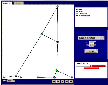
1. The basic coalescent. The Fisher-Wright model assumes a non-sexually reproducing organism. What happens if there is mixing via genetic recombination? Select the “recombination” link after choosing the Hudson animator, or make sure the ‘recombination’ pull-down menu item is selected. Choose n=5 sequences and rho=0 (no recombination). Press recalc and the animation starts. The speed can be controlled via the “speed” item on the bottom-left corner, or you can just fast-forward as before. Details regarding each node, e.g., the scaled time to coalescence, can be viewed in the small window at the right when moving the mouse over the relevant node. Clicking on the ‘trees’ panel will untangle the trees, as before.
a. What is the time to the first coalescence event? Write it down.
b. What is the time to the most recent common ancestor? Write it down.
c. Repeat (a) and (b) 5 times (by pressing recalc). How does the time to first coalescence and time to most recent common ancestor vary?
2. Repeat with n= 10 and n=20 sequences. What are the times to the first coalescence and the most recent common ancestor in these cases? Write this down for 5 different runs.
The recombination rate is determined by rho=2nc, where c is a constant. In the animation, recombination events are marked as blue nodes (in contrast to the green nodes of coalescent events). Now we’ll see what the mixing effect of recombination does to genealogy trees.
4. Set n=5, and rho=1. Press recalc and study the animation. Do any recombination events occur? These will be marked by blue nodes, along with a crossing line to the other individual with whom the recombination occurred. Also, if you mouse over the blue node, you’ll see what ‘fraction’ of that individual’s ‘genetic’ material that was exchanged (see picture below). If not, try again. Try a total of 5 times and write down the number of recombination events in each case. Examine where in the sequence recombination events occur.
a. Are there any examples where a different part of the sequence of ‘individuals’ has different most recent common ancestors (MRCAs, marked in green) at different time points? Why would this be possible?
b. Can you find any examples of “trapped” non-ancestral material (colored white) between blocks of ancestral material?
c. Try to press the ‘trees’ tab. Here it is possible to study each of the different trees over the sequence. How many different trees are there and how does this relate to the number of recombination events? Try to find examples of each of the following recombination types:
i. Recombination changing the topology of the tree
ii. Recombination changing the branch length but not the topology of the tree
iii. Recombination that does not change the tree
What is the total number of each of types i, ii, and iii during the 5 replicate runs?
5. Try setting rho=2 and n=10
a. How many recombinations occur now?
b. At which time do different parts of the sequence find a most recent common ancestor?
c. At which time have all the different parts of the sequence found a most recent common ancestor? Compare this time with the time to most recent common ancestor without recombination.
5. Try setting rho=5 and n=20. How many recombination events occur now? How many different most recent common ancestors are there over the sequence now?
Discuss in a few sentences the implications
Coalescent with exponential growth
Now choose the coalescent animation with exponential growth selected on the pull-down menu. This is controlled with the parameter exp, which is equal to Nb. This parameter measures how many times the present population is larger than the population 2N, where N= the size of the present day population. For humans, all estimates suggest that exp>100.
6. Try to simulate n=10 sequences and different runs with exp=1, 10, 100, 1000
a. How does the shape of the genealogical tree depend on the value of exp?
b. How can that be?
Part 2: Detecting selection – simple methods
Part 2.1 Detection of selection in primate lysozyme enzymes
Already-aligned lysozyme C precursor DNA sequences from different species of apes (including human) in FASTA format may be found here. Analyze the pattern of nonsynonymous and synonymous substitutions between these genes. Use the SNAP utility.
1. Using the nonsynonymous/synonymous ratio test, is there any evidence for positive selection on the lyz C gene in ape-like primates?
2. What is the overall dN/dS ratio for the lyz C genes in the alignment? Is there an excess of silent or coding mutations?
3. Are the phylogenetic trees based on dN and dS different? What do you think this means?
4. Discuss the results of this analysis. Why might the lyz C genes among these species differ? Can natural selection be responsible? (Reference: Polley SD, Conway DJ. 2001. Strong diversifying selection on domains of the Plasmodium falciparum apical membrane antigen 1 gene. Genetics. 158:1505-1512.)
Part 2.2 Detection of selection with Tajimas's D test
Fetch this sequence alignment of Plasmodium falciparum (malaria) apical membrane antigen 1 gene sampled according to several sources (here) and save the sequences on your local computer. (For the next part we assume that you all have access to PCs running Windows…if not, see me.) Download and install DnaSP on your local PC. This file is a self-extracting, and you just run it to install the program itself. You will use the program to analyze nucleotide diversity and test selection with respect to this dataset via “Tajima’s D” using a sliding window of appropriate size. “Tajima’s D” tests the statistical significance of an excess of common as compared to rare nucleotide variants, via the difference between two different estimates of nucleotide diversity. Under the neutral model, i.e., constant population size and no selection, we can set one estimate as θ= 4Nμ. We can make a second estimate of nucleotide diversity as π= the sum of the number of nucleotide differences between the ith and the jth DNA sequences. D is simply π-θ, and the null hypothesis is that this value is 0. Departures from 0 indicate that the underlying assumptions might be incorrect – i.e., a negative value of D indicates either purifying selection or population expansion, while positive values of D indicate positive selection.
You can use DnaSP as follows:
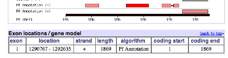
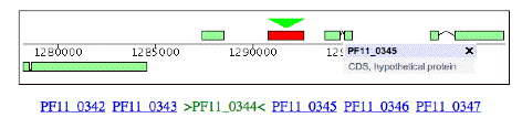
Here is some information on this gene, P. falciparum PF11_0344, an apical membrane precursor, 622 amino acids long. It resides on Chromosome 11 of P. falciparium, spanning locations 1290767 – 1292635. I have placed a link to the NCBI entry on this gene and a link to the plasmodium database entry for this gene below. You can use these links to view the gene’s amino acid sequence, nucleotide sequence, and even the 3-D structure of part of the corresponding protein (structure 1HN6). Some snapshots from the plasmodium database are below. Perhaps the best description is the link that follows, from the Sanger Center, which gives a good overview of the functioning of the protein associated with this gene and a great browser view.
Link 0: Sanger Center Plasmodium falciparum database
Link 1: NCBI genome database
Link 2: Plasmodium database
Link 3: 3-D structure PDB database
Link 4: Conserved Domain Database (CDD) at NCBI
Chromosome 11 picture:
Gene AA sequence:
![]()
The amino acid sequence for this gene is as follows (from NCBI):
1 mrklycvlll safeftymin fgrgqnyweh pyqnsdvyrp inehrehpke yeyplhqeht
61 yqqedsgede ntlqhaypid hegaepapqe qnlfssieiv ersnymgnpw teymakydie
121 evhgsgirvd lgedaevagt qyrlpsgkcp vfgkgiiien snttfltpva tgnqylkdgg
181 fafppteplm spmtldemrh fykdnkyvkn ldeltlcsrh agnmipdndk nsnykypavy
241 ddkdkkchil yiaaqenngp rycnkdeskr nsmfcfrpak disfqnytyl sknvvdnwek
301 vcprknlqna kfglwvdgnc ediphvnefp aidlfecnkl vfelsasdqp kqyeqhltdy
361 ekikegfknk nasmiksafl ptgafkadry kshgkgynwg nyntetqkce ifnvkptcli
421 nnssyiatta lshpievenn fpcslykdei mkeiereskr iklndnddeg nkkiiaprif
481 isddkdslkc pcdpemvsns tcrffvckcv erraevtsnn evvvkeeykd eyadipehkp
541 tydkmkiiia ssaavavlat ilmvylykrk gnaekydkmd epqdygksns rndemldpea
601 sfwgeekras httpvlmekp yy
The full ORF sequence (so far) of the entire falciparum chromosome 11 may be found here.
(This includes just predicted ORFs larger than 50 amino acids long.)
The full nucleotide sequence for gene AMA1 (PF11_0344) may be found here.
Part 2.3. Volatility. Given this information, we can now test in a noncomparative way whether this gene is under positive selection: you can use J. Plotkin’s volatility server, and run it over all of the ORFs in chromosome 11 to see whether the PF11_0344 gene stands out. (The server takes fasta format as input, so you can use the chromosome 11sequence in the lab directory, above.) Please go ahead and do this now. Go to the volatility server and upload the entire chromosome 11 sequence. What should the kappa (transition/transversion rate ratio) be? (Click on the ‘About kappa’ box. See if you can figure out how to use DnaSP to estimate kappa, or do a bit of research on how this is done.) After you run the program, you can download the result to an excel spreadsheet locally. Then you’ll have to do a bit of grepping to find the AMA1 gene (but it’s not that hard). See what its computed volatility is – does it agree with your previous analysis from section 2.2? What do you think this means?
Part 2.4. Going further. Let’s do a bit more digging on this one – a more open-ended question. The analysis in section 2.2 looked at parts of a single gene, while the volatility analysis compares whole genes against the rest of a genome. See if you can use DnaSP to locate the regions within the gene that seem to be undergoing selection, and look at which amino acid residues they correspond to. Can you locate them in the actual 3-D structural map that the PDB provides? (I know you might have to ask your resident bioinformatics person in class about some of the details about how to do this, or the biochemistry – that is OK – just do your best and please work together.)
Part 3. Detecting selection – likelihood methods (PAML)
Part 3.1
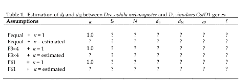
In this exercise, we shall use likelihood methods to test the sensitivity of dN/dS, aka ‘omega’, with respect to basic evolutionary assumptions about codon evolutionary changes.
Dataset: GstD1 genes of Drosophila melanogaster and D. simulans (600 codons). This data file is located here.
Objective 1: Test the effect of transition / transversion ratio (kappa, orκ) on dN/dS (Note that you use this ratio when you employ J. Plotkin’s volatility analysis. Hmm - perhaps you can use this estimation in the previous problem.)
Objective 2: Test the effect of codon evolutionary change differences (πI’s).
Your goal will be to fill in the following table, which displays six rows, corresponding to six possible combinations for kappa and pi:
All codon frequency changes equal (denoted Fequal), and kappa = 1.
All codon frequency changes equal, and kappa estimated by maximum likelihood from the actual data
Codon frequencies estimated via a Jukes-Cantor 3x4 redundancy class matrix, and kappa = 1
Codon frequencies estimated via a Jukes-Cantor 3x4 matrix, and kappa estimated from the data
Full 61x61 codon frequency matrix, and kappa = 1
Full 61x61 codon frequency matrix, and kappa estimated from the data
(See the Lewontin paper for further discussion of these codon evolution matrices.)
Terminology:
κ= transition/transversion rate ratio
S = number of synonymous sites
N = number of nonsynonymous sites
ω= dN/dS
ℓ= log likelihood score (selection vs. no selection)
Your filled in table should be something like this, with numbers replacing the question marks:
The general PAML web page may be found here.
You can read the documentation file (rather opaque) here.
The actual PAML site has an FAQ that is worth reading if you want to really delve into things, or seek more clarification.
The control data file for the PAML program (see web page here – download and edit).
---------------------- beginning of file -------------------------
seqfile = seqfile.txt * (DNA) sequence data filename (replace)
outfile = results.txt * main result file name (replace w/ yours)
noisy = 9 * 0,1,2,3,9: how much output on screen
verbose = 1 * 1:detailed output
runmode = -2 * -2:pairwise comparison
seqtype = 1 * 1:codons
CodonFreq = 0 * 0:equal,1:F1X4,2:F3X4,3:F61
model = 0 *
NSsites = 0 *
icode = 0 * 0:universal code
fix_kappa = 1 * 1:kappa fixed, 0:kappa to be estimated *
kappa = 1 * fixed or initial value
fix_omega = 0 * 1:omega fixed, 0:omega to be estimated
omega = 0.5 * 1stfixed omega value
* Uncomment out the various lines below to get the various combos
* Codon bias = none; Ts/Tv bias = none
* Codon bias = none; Ts/Tv bias = Yes (ML)
* Codon bias = yes (F3x4); Ts/Tv bias = none
* Codon bias = yes (F3x4); Ts/Tv bias = Yes (ML)
* Codon bias = yes (F61); Ts/Tv bias = none
* Codon bias = yes (F61); Ts/Tv bias = Yes (ML)
--------------- end of control file input -------------------------
Discuss your findings with respect to the sensitivity of the analysis to various assumptions about nucleotide changes – do the assumptions make a difference in this case? ‘
Part 2. Likelihood ratio test method for detecting variation in seletion pressure among branches in a phylogenetic tree.
Example: The lactate dehydrogenase (Ldh) gene family is an important model system for investigating the molecular evolution of isozyme multigene families. The rate of evolution for Ldh is known to have increased in the form Ldh-C following a gene duplication event. (See reference: Lactate dehydrogenase (LDH) gene duplication during chordate evolution: the cDNA sequence of the LDH of the tunicate Styela plicata. Stock DW, Quattro JM, Whitt GS, Powers DA., Mol Biol Evol.1997 Dec.14(12):1273-84).
You can take the following tree as indicative of hypotheses we would like to investigate:
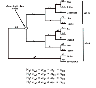
Here we hypothesize that the ancestral form duplicated into two types: Ldh-A and Ldh-C. We want to use PAML to see if we can answer the following questions:
1. Was there an increase in the underlying mutation rate of Ldh-C?
2. Has there been increased positive selection following the duplication event?
3. Has there been a long term change in selection pressure?
These are all questions regarding the relative differences among selection between different branches of this presumed phylogenetics tree. Using PAML, we want to compare the relative selection pressure on these two branches via a likelihood ratio test – what PAML calls a ‘branch specific’ codon model. We need to set up a set of models that test whether dN/dS along one branch is the same as another branch or not.
To do this, we first divide the tree into two C sections, C0 and C1, and two A sections, A0 and A1, as indicated above. We next set up four hypotheses, H0 , H1, H2, and H3, that make assumptions about the relative values of dN/dS among these four tree components. For example, the null hypothesis, H0 , asserts that the dN/dS ratios (omega values) along all branches are equal – i.e., no change in evolutionary rates after duplication. In PAML, we use the control file parameter model=0 to test this hypothesis that all rates are equal (see the control file below). Against this hypothesis we test the claims that (H1) the ratio along C0 (along the line after the presumed duplication) differs from the others; that (H2) the C lineage rate (C0 and C1) as a whole is different from the A side of the tree (A0 and A1); and (H3) A1 and C0 are both different from A0 and C1.
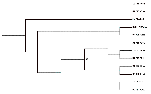
In order to do this analysis in PAML, we must supply a tree structure file along with our usual control file and sequence file. Such PAML analyses require branch-specific codon models to allow different branch groups to have different ωs, leading to so-called “two-ratios” and “three-ratios” models. All those models require branches or nodes in the tree to be labeled. Branch labels are specified via the symbol “#” placed in a parenthesis-notation format for the tree structure. The branch labels are consecutive integers starting from 0, which is the default and does not have to be specified. For example, the following tree:
((Hsa_Human, Hla_gibbon)#1,((Cgu/Can_colobus,Pne_langur), Mmu_rhesus),(Ssc_squirrelM, Cja_marmoset));
has a branch label #1 for fitting models of different ω ratios for branches. The internal branch ancestral to human and gibbon has the ratio ω1, while all other branches (with the default label #0) have the background ratio ω0. This fits the model in table 1C for the small data set of lysozyme genes in Yang (1998). (See the readme file for PAML here.)
Yes, this is incredibly baroque and brain-dead. In fact, you really don’t have to understand this notation to do the problem – the tree files are already provided for you. An easy way to visualize the parenthesis structure (if you are not used to Lisp), is to simply input the tree description file into the program treeview, which is on your CD-ROM. This is how we produced the pictures for the different hypotheses below.
Here is the first part of the control file for the relevant codeml program:
seqfile = seqfile.txt * sequence data filename (replace w/ actual seq)
treefile = tree.txt * tree structure file name (replace w/ tree file)
outfile = results.txt * main result file name
noisy = 9 * 0,1,2,3,9: how much rubbish on the screen
verbose = 1 * 1:detailed output
runmode = 0 * 0:user defined tree (so you need to input a tree file)
seqtype = 1 * 1:codons
CodonFreq = 2 * 0:equal, 1:F1X4, 2:F3X4, 3:F61
model = 0 * 0:one omega ratio for all branches
* 1:separate omega for each branch
* 2:user specified dN/dS ratios for branches
NSsites = 0 *
icode = 0 * 0:universal code
fix_kappa = 0 * 1:kappa fixed, 0:kappa to be estimated
kappa = 2 * initial or fixed kappa
fix_omega = 0 * 1:omega fixed, 0:omega to be estimated
omega = 0.2 * initial omega
------------ end of control file ------------------------------------
Start by specifying model=0, which sets all omega values the same on each branch, i.e., hypothesis H0. You must also input the tree file as specified in the control file. For the next 3 runs, you should set model=2, i.e., user specified omega values (dN/dS ratios) for specified branches in the phylogenetics tree. For these 3 runs you therefore provide a slightly different tree input file that says exactly where the dN/dS ratios are to be compared. These files are already in the lab directory for you to use:
Ldhcodeml sequence file: (TXT)
Tree H0 file: (TXT)
Tree H1 file: (TXT)
Tree H2 file: (TXT)
Tree H3 file (TXT)
Tree format for model H1:
(X02152Hom,U07178Sus,
(M22585rab,
((NM017025Rat,U13687Mus),
(((AF070995C,(X04752Mus,U07177Rat)),
(U95378Sus,U13680Hom))#1,(X53828OG1,U28410OG2)))))
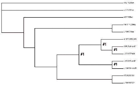
Picture of model H2. Note how this lumps all the “C” lineage together, and tests that omega value against the “A” lineage.
(X02152Hom,U07178Sus,
(M22585rab,
((NM017025Rat,U13687Mus),
(((AF070995C #1,(X04752Mus #1,U07177Rat #1)#1)#1,
(U95378Sus #1,U13680Hom #1)#1)#1,
(X53828OG1,U28410OG2)))))
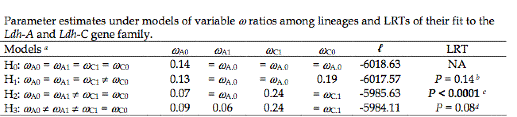
Your job is to run these analyses to fill in the following table where the ‘blank’ values are and confirm (or not), the questions that were given at the beginning of this section.

![]()
![]()
![]()
![]()
![]()
Part 4: Application to Yeast (tbd)