
The graph of the exponential distribution is shown in Figure 1.
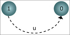
Figure 1: Graph of Markov Process for Exponential Distribution. (Figure by MIT OpenCourseWare.)
The transition equations are
\[ p(0,t + \delta t) = \mu \delta tp(1,t) + p(0,t) + o(\delta t) \tag 1 \]
\[ p(1,t + \delta t) = (1 - \mu \delta t) p (1,t) + (0)p (0,t) + o(\delta t) \tag 2 \]
or,
\[\frac{dp(0,t)}{dt}= \mu p(1,t) \tag 3 \]
\[\frac{dp(1,t)}{dt}= -\mu p(1,t) \tag 4 \]
Solve differential equations (3), (4) and we get
\[p(0,t) = 1 - e^{-\mu t}\tag 5\]
\[p(1,t) = e^{-\mu t}\tag 6\]
Function \(p(0,t)\) is actually the cumulative density function of the exponential distribution
\[F(t) = p(0,t)\tag 7\]
Then the density function of the exponential distribution is
\[f(t) = \frac{dF(t)}{dt}= \mu e^{- \mu t}\tag 8\]


