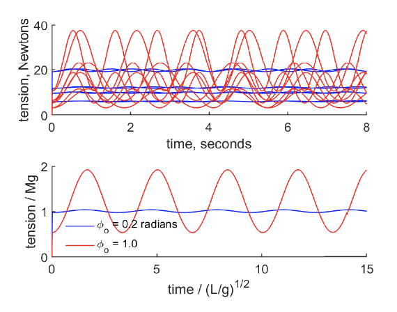
Tension in the line of a simple pendulum. (Image courtesy of the instructor.)
This essay describes a three-step procedure of dimensional analysis that can be applied to all quantitative models and data sets. In rare but important cases, the result of dimensional analysis will be a solution; more often the result is an efficient way to display a large or complex data set.
The first step of an analysis is to define an appropriate physical model, which is nothing more than a list of the dependent variable and all of the independent variables and parameters that are thought to be significant. The premise of dimensional analysis is that a complete equation made from this list of variables will be independent of the choice of units. This leads to the second step, calculation of a null space basis of the corresponding dimensional matrix. (A computer code is made available for this calculation.) To each vector of the null space basis there corresponds a nondimensional variable, the number of which is less than the number of dimensional variables. The nondimensional variables are themselves a basis set and in most cases their form is not determined by dimensional analysis alone.
The third and, in some respects, most interesting step is to choose an optimal form for the basis set. One very useful strategy is to nondimensionalize the dependent variable by a physically motivated “zero order” solution. When carried to completion, this leads naturally to a scaling analysis in which the nondimensional variables of a model equation are O(1) in some relevant limit. Scaling analysis is often an essential first step in an approximation method. The remaining nondimensional variables can then be formed in ways that define the geometry of the problem or that correspond to the ratios of terms in a model equation, e.g., the Reynolds number or Froude number often arise in models of geophysical fluid dynamics.
Online Textbook
Dimensional Analysis of Models and Data Sets: Similarity Solutions and Scaling Analysis (PDF)
Appendix: Draining a Tank (PDF)


