< Previous lab day | Module 2 lab index | Next lab day >
Introduction
Today you will obtain titration curves against calcium for your wild-type and mutant proteins using an automated fluorescence plate reader. This machine reads multiple samples in a standard format – in our case, a 96-well microtiter plate. The output is a grid of up to 96 fluorescence values, for rows A-G and columns 1-12, which is amenable to analysis with a program like Excel.
In order to further benefit from this high-throughput testing format, you will make friends with the multichannel pipet, a purely mechanical rather than digital aid for repetitive experiments. This tool allows you to suck up and expel equivalent volumes of multiple identical samples (usually 8-12 at a time) with just one stroke. You will use this type of pipet to fill each row of a microtiter plate with one type of protein sample, and each column with a different concentration of calcium. Although a multichannel pipet can be sufficient for a typical research lab, in pharmaceutical companies that may be assaying thousands of samples a day, yet more steps of automation and scaling up are required, such as robotic pipet arms that obviate the need for manual pipetting at all. The degree of automation commercially available, or developed ‘in-house’ in a certain lab or corporation, depends in part on the frequency with which a certain assay is used. Assays used by many different labs and companies (such as fluorescence or absorbance spectrophotometry) are likely to breed commercially available high-throughput machines.

Signal:noise in arbitrary data collection. Background measurements (open circles), sample measurements (closed circles), and average values (short horizontal lines) are shown. The short line without any data points represents the reduction in average signal when background is subtracted. All measurements are with respect to an arbitrary vertical axis; the long horizontal line represents a measurement of zero.
While the concept of scale is a pragmatic concern, a perhaps more substantive topic of interest to us today is that of confidence in our results. As you are probably well-aware, every manipulation and measurement you make in the lab has an error associated with it. For example, consider the ubiquitous P200 pipetman. According to one pipet manufacturer, its accuracy is 1% (slightly worse at the lowest volumes). So an attempt to pipet 100 μL would result in an actual volume of 99-101 μL from the error of the instrument alone, which could be further compounded by a sleepy pipet operator, say. The precision of a pipet is typically better than its accuracy, 0.25% for the example given above. Precision refers to the reproducibility of a given measurement, not its absolute accuracy. This simple example demonstrates the general principles applicable to other types of error.
You will attempt to get a sense of the overall error of today’s experiment by running your protein samples in duplicate. That is, for each protein-calcium combination, you will perform two independent measurements. These measurements can then be averaged to smooth out your data, and hopefully improve the signal to noise ratio - where signal here refers to true differences between samples mixed with different amounts of calcium, and noise means inherent fluctuations in the system due to error. Noise in this experiment can also refer to background fluorescence of the sample buffer. Thus, another way to maintain a reasonable signal:noise ratio is by keeping our protein fairly concentrated, so that the absolute fluorescence values we obtain are high compared to the background. The figure at right demonstrates the above concepts. Scatter in the data (not all of the circles are at the same height) is one kind of noise. The level of background is another kind of noise: the left-hand data has a relatively low signal and thus poor signal:noise ratio, while the right-hand data has a relatively high absolute signal and improved signal:noise ratio.
Protocols
Only 2-3 groups at a time will work in lab today. Last time you should have signed up for a one-hour block.
Part 1: Protein Gel Observation
If you would like to, take a look at your Coomassie-stained gel from the previous lab.
Tips for Success
Take great care today to limit the introduction of bubbles in your samples. When expelling fluid, pipet slowly while touching the pipet tip against the bottom or side of the well. When using the multichannel pipet, always check to make sure all tips are getting filled - sometimes one tip may not be on all the way, and will pull up less volume than the others. If this happens, release the fluid, adjust the tip, and try again.
Protocol

Titration sample preparation.
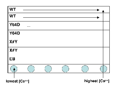
- Take a black 96-well plate, and familiarize yourself with the scheme at right: top two rows are wild-type, next two rows are the M124S mutant, and the final two are your own mutant.
- The dark sides of the plate reduce “cross-talk” (i.e., light leakage) between samples in adjacent wells, another potential contribution to error.
- Transfer an aliquot of wild-type protein to a plastic reservoir. Use the multichannel pipet to add 30 μL of protein (per well) to the top two rows of your plate.
- Take a fresh reservoir, and repeat step 2 for your mutant proteins, adding each one to the appropriately labeled rows.
- Finally, add plain EB buffer (no protein) to the seventh row of the plate, using the shared dedicated reservoir. (Why do you think we are including a protein-free row of solutions?)
- Using shared reservoir 1 (lowest calcium concentration), add 30 μL to the top seven rows in the first column of the plate. Discard the pipet tips.
- Now work your way from reservoirs 2 to 12 (highest calcium concentration), and from the left-hand to the right-hand columns on your plate. Be sure to use fresh pipet tips each time! If you do contaminate a solution, let the teaching faculty know so they can put out some fresh solution.
- Finally, cover the plate with parafilm and wrap it in aluminum foil.
Part 3: Fluorescence Assay
- BPEC (the Biological Process Engineering Center) has graciously agreed to let us use their plate reader. Walk over to the BPEC instrument room with a member of the teaching staff.
- You will be shown how to set the excitation (485 nm) and emission (515 nm) wavelength on the plate reader to assay your protein.
- Your raw data will be posted or emailed to you; alternatively, you can bring your own flash drive to recover the data immediately.
For Next Time
- Prepare a figure and caption for your SDS-PAGE results. Look up the expected molecular weight using the IPC sequence document and this online Protein Molecular Weight tool (or similar) Web site. Be sure to add ~ 3 KDa for the size of the N-terminus of pRSET (His tag, etc). If you see two strong bands, what do you think the second one is? This homework will be graded during class next time so you can incorporate any comments in your final report.


