
1.225J Transportation Flow Systems Quiz (PDF version also available)
Duration: 3 hours
Student Name:_____________________ Alias:___________________
Instructions
- This exam is open-book.
- No cooperation is permitted.
- Please write down your name and an alias, which we may need in emailing you your grades.
- Please write down your answers in the reserved space. Please provide concise answers, and do not be surprised if answers are not more than one to three sentences long.
| QUESTIONS | POINTS |
|---|---|
| Question 1 | /25 |
| Question 2 | /15 |
| Question 3 | /20 |
| Question 4 | /25 |
| Question 5 | /15 |
| Total | /100 |
Question 1 (25 points): Capacity Models of Runways and Highways
1.1 (7 points) Consider the analytical model of the capacity of one runway developed in Lecture 2. Let W be a constant greater than 1. Assume that the runway occupancy times are negligible. Assume you have been assigned the task to assess two alternative proposals to improve the capacity of a runway: (P1) multiply the final approach speeds of all aircraft types by W, or (P2) divide the length of the final approach path by W. In any given proposal, with the exception of the proposed changes, everything else in the model remains constant.
Would the two proposals lead to the same improved runway capacity? If not which of the two proposals would lead to the lowest runway capacity? Please justify your answer using the analytical model of the runway capacity.
1.2 (6 points) Consider a queuing system with one server and infinite capacity. Customers arrive with exponentially distributed inter-arrival times at an average rate of customers per hour. The average service rate is customers per hour. The distribution of service time is not known. Denote by W1 and W2 the respective waiting times in the queuing system, if the service time were to follow exponential and deterministic distributions. Using an intuitive argument, and without computing W1 and W2, compare the waiting time in the queuing system to W1 and W2.
1.3. (6 points) Three variables describe traffic flow on a road segment: the density k (vehicles per kilometer), the speed u (kilometers per hour) and the flow rate q (vehicles per hour). These three variables are interrelated through the following two relations: a generic relation q=uk and a link-specific function relating u to k. Denote by kj is the jam density of a one lane highway. On a three lane highway, the u vs. k relation is given by: If k<=k*, u= 100, and if k>=k*, u= 20 ((3kj/k)-1). The maximum flow per three lanes is 5400 vehicles per hour. Please draw the fundamental diagram of this three-lane highway.
1.4 (6 points) Consider a stretch of a highway with a two-lane portion, followed by a three-lane portion. The point of juncture of these portions is called an expansion. The maximum flow that can pass through the expansion is 3600 vehicles per hour. Assume that the model described in question 1.3 is an accurate description of highway flows, densities and speeds. We are interested in the value of the density k over the three-lane highway, immediately after the juncture point. Show that the value of k cannot be in an interval (k1, k2), where k1 and k2 are two particular density values [determine k1 or k2, or locate them on the fundamental diagram].
Question 2 (15 points)
In this question consider the following non-congested network. The number near each link denotes the link travel time. Assume that the origin-destination demands from nodes 2, 3, 4 and 5, to node 1, are respectively 1, 2, 2, and 5.
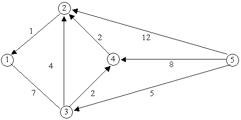
2.1 (8 points) Using Dijkstra’s shortest path algorithm, solve for the shortest paths from all other nodes to node 2. Please show the details of your calculations on the above Figure depicting the network. Also, please show the obtained shortest path tree in the space below.
2.2 (7 points) Assume that we want to assign the above origin-destination demand to the network such that the total travel time is minimized. Using your answer to Question 2.1, please provide a solution to this system-optimal traffic assignment example. If the solution is not unique, please provide another optimal solution.
Question 3 (User Optimal vs. System Optimal) (20 points)
Assume you are assigned to perform static traffic assignments for networks in which link travel times are modeled using Davidson’s volume delay function. The travel time of a link is then given by a function of the form:
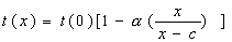 ,
,
where x is the flow rate on the link, c is the link capacity, t(0) is the free flow travel time, and  is a link parameter ( is a real non-negative (can be equal to zero) number).
3.1 (4 points) Consider a simple network with two nodes linked by two parallel arcs. The travel time functions of links 1 and 2 are respectively given by:
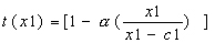 , and
, and
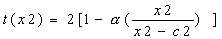 .
.
We are interested in assigning a travel demand q between these nodes according to the User-Optimal principle. Depending on the value of q, one or two links will be used. Please provide the intervals of demand values q corresponding to the following two cases: one link is used, and both links are used. Please justify your answer.
3.2 (4 points) Consider the interval of values of q when both links carry positive flows in the user-optimal traffic assignment corresponding to the small network described in Question 3.1. Provide a system of equations the solution of which are the link flows x1 and x2 (Do not solve the system of equations).
3.3. (7 points) A static traffic assignment package is available to you to solve static traffic assignment problems. This specialized package however solves only for User-Optimal traffic assignment solutions. If one wants to solve a System Optimum static traffic assignment, one must then transform it to an equivalent UO problem that can then be solved by this package. The transformation consists in using different link performance functions corresponding to Davidson’s functions.
What modified link travel time functions, corresponding to the real link performance functions
 ,
,
would you use in order for the UO traffic assignment package to give you the solution to the SO traffic assignment problem.
3.4 (5 points) For which value (or values) of parameter, is a User Optimal traffic assignment solution also a System Optimal traffic assignment solution?
Question 4 (25 points)
Consider a queuing system with 1 server and infinite capacity. Customers arrive with exponentially distributed inter-arrival times at an average rate of  customers per hour. Let k be a given real-number greater than or equal to 1. The service time is exponentially distributed with an average service rate depending on the number of customers in the system. When there are n customers in the system, the service rate is
vehicles per hour. Denote by ρ the ratio  .
.
4.1 (2 points) Show that the service rate is in the interval [m, km] for all values of n.
4.2 (2 points) Assume that l < m. The minimum average service rate is then greater than the average arrival rate. Intuitively, explain why there is a non-zero probability that there will be customers who would have to wait after they arrive before they are admitted for service.
4.3 (7 points) Draw the state-transition diagram of this queuing system.
4.4 (7 points) Please write down, but do not solve, the set of equations that you would use to solve for W, Wq , Lq, and L (We just want to know the equations that you would use and the order in which you will solve them).
4.5 (2 points) Is the condition l < m (or r\\<1) sufficient in order to have the steady-state condition? Please give a one to two sentences justification of your answer.
4.5 (2 points) Consider the case when k>1. Intuitively could the queuing system be in steady state if r is slightly greater than 1?
4.6 (3 points) Assume that r >=k. After a large enough (approaching infinity) number of customers arrived at the queueing system , what would be the length of the queue? No calculations are necessary.
Question 5 (15 points)
In Queuing models for which analytical expressions of the fundamental queuing variables have been derived, inter-arrival times are usually assumed to follow a negative-exponential distribution. In many circumstances, especially in transportation systems, arrivals can be scheduled and hence inter-arrival times may not follow the negative-exponential distribution.
In this question we first consider a queuing model with two services and infinite capacity. The service time is exponentially distributed. The average service rate of each server is . The intervals between arrivals is distributed in interval [1,11], with density function
f(t)=0.05+0.01*(t-1),
where t is in interval [1,11].
We want to develop an event-based simulation of this queuing system. Assume the notation of Lecture 9: An: arrival time of customer n, Dn: departure time (service completion time) of customer n. Hn: inter-arrival (arrival headway) time of customer n and Sn: service time of customer n.
5.1 (1 point) What is the code of this queuing system?
5.2 (2 points) Show that the cumulative distribution of the inter-arrival time is given by:
0.05(t-1)+0.005(t-1)^2.
5.3. (2 points) For a given random number r, give an equation that allows us to determine a random observation H(r) of the inter-arrival time. (Please do not solve the equation).
5.4. (3 points) Express Dn as a function of An, Dn-1, and Dn-2.
5.5 (4 points) Please provide the expressions for quantities that would allow one to develop an event-based simulation model of this queuing system.
5.6 (3 points) If you have now k servers, each with an average service rate of , what minimal changes would you make to the expressions derived in 5.2 to model this modified queuing model? [The inter-arrival times are the same as in questions 5.1-5.5]


