
.toc { margin-left: 2em; } .lecslide { margin-top: 1em; margin-bottom: 1em; border-top: 0.5px solid #808080; padding-top: 1em; text-align: center; } .lecslideimg { width: 5in; border: 1px solid black; }
- Beta ISA Summary
- Programming Languages
- Assembly Language
- Example UASM Source File
- How Does It Get Assembled?
- Registers Are Predefined Symbols
- Labels and Offsets
- Mighty Macroinstructions
- Assembly of Instructions
- Example Assembly
- UASM Macros for Beta Instructions
- Pseudoinstructions
- Factorial with Pseudoinstructions
- Raw Data
- UASM Expressions and Layout
- Summary: Assembly Language
- Universality?
- Models of Computation
- FSM Limitations
- Turing Machines
- Other Models of Computation
- Computability?
- Turing Machines Galore!
- The Universal Function
- Universality
- Turing Universality
- Coded Algorithms: Key to CS
- Uncomputability!
- Why fH is Uncomputable
Content of the following slides is described in the surrounding text.
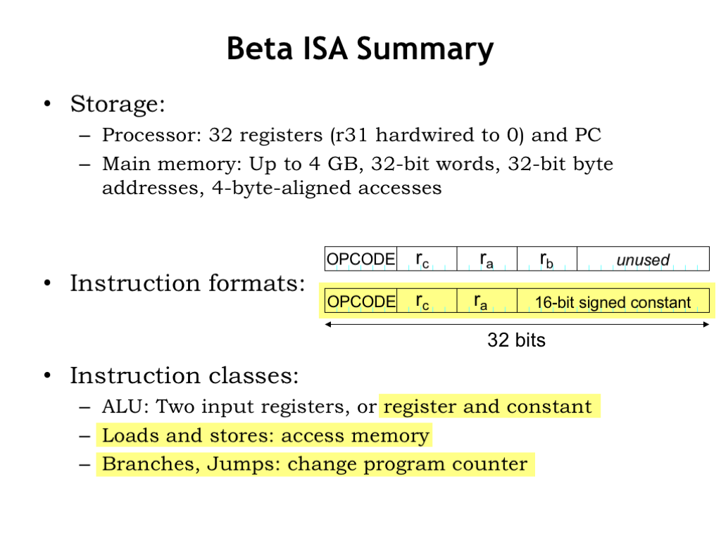
In the previous lecture we developed the instruction set architecture for the Beta, the computer system we’ll be building throughout this part of the course. The Beta incorporates two types of storage or memory. In the CPU datapath there are 32 general-purpose registers, which can be read to supply source operands for the ALU or written with the ALU result. In the CPU’s control logic there is a special-purpose register called the program counter, which contains the address of the memory location holding the next instruction to be executed.
The datapath and control logic are connected to a large main memory with a maximum capacity of \(2^{32}\) bytes, organized as \(2^{30}\) 32-bit words. This memory holds both data and instructions.
Beta instructions are 32-bit values comprised of various fields. The 6-bit OPCODE field specifies the operation to be performed. The 5-bit Ra, Rb, and Rc fields contain register numbers, specifying one of the 32 general-purpose registers. There are two instruction formats: one specifying an opcode and three registers, the other specifying an opcode, two registers, and a 16-bit signed constant.
There three classes of instructions. The ALU instructions perform an arithmetic or logic operation on two operands, producing a result that is stored in the destination register. The operands are either two values from the general-purpose registers, or one register value and a constant. The yellow highlighting indicates instructions that use the second instruction format.
The Load/Store instructions access main memory, either loading a value from main memory into a register, or storing a register value to main memory.
And, finally, there are branches and jumps whose execution may change the program counter and hence the address of the next instruction to be executed.
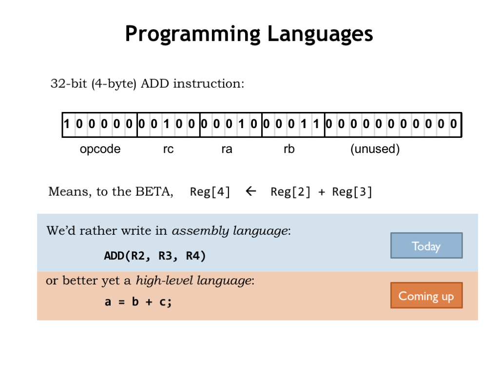
To program the Beta we’ll need to load main memory with binary-encoded instructions. Figuring out each encoding is clearly the job for a computer, so we’ll create a simple programming language that will let us specify the opcode and operands for each instruction. So instead of writing the binary at the top of slide, we’ll write assembly language statements to specify instructions in symbolic form. Of course we still have think about which registers to use for which values and write sequences of instructions for more complex operations.
By using a high-level language we can move up one more level abstraction and describe the computation we want in terms of variables and mathematical operations rather than registers and ALU functions.
In this lecture we’ll describe the assembly language we’ll use for programming the Beta. And in the next lecture we’ll figure out how to translate high-level languages, such as C, into assembly language.
The layer cake of abstractions gets taller yet: we could write an interpreter for say, Python, in C and then write our application programs in Python. Nowadays, programmers often choose the programming language that’s most suitable for expressing their computations, then, after perhaps many layers of translation, come up with a sequence of instructions that the Beta can actually execute.
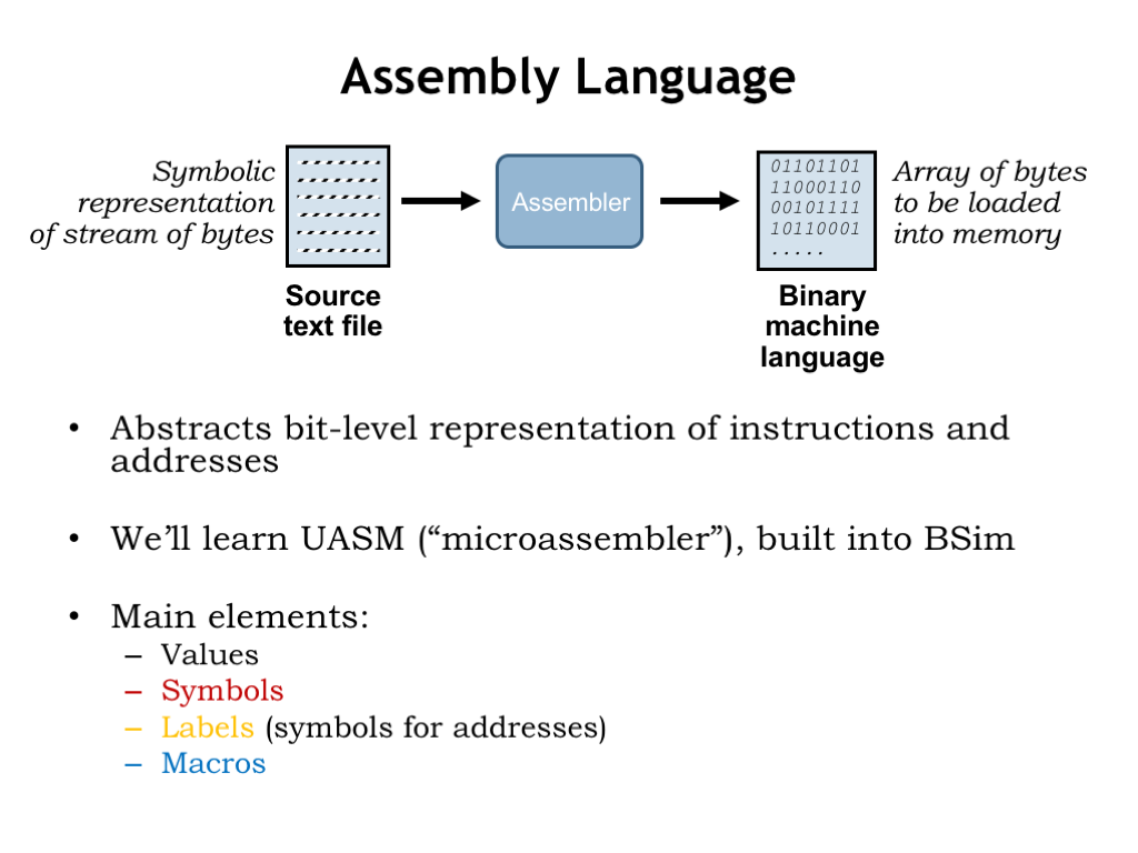
Okay, back to assembly language, which we’ll use to shield ourselves from the bit-level representations of instructions and from having to know the exact location of variables and instructions in memory. A program called the “assembler” reads a text file containing the assembly language program and produces an array of 32-bit words that can be used to initialize main memory.
We’ll learn the UASM assembly language, which is built into BSim, our simulator for the Beta ISA. UASM is really just a fancy calculator! It reads arithmetic expressions and evaluates them to produce 8-bit values, which it then adds sequentially to the array of bytes which will eventually be loaded into the Beta’s memory. UASM supports several useful language features that make it easier to write assembly language programs. Symbols and labels let us give names to particular values and addresses. And macros let us create shorthand notations for sequences of expressions that, when evaluated, will generate the binary representations for instructions and data.
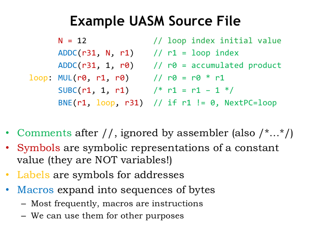
Here’s an example UASM source file. Typically we write one UASM statement on each line and can use spaces, tabs and newlines to make the source as readable as possible. We’ve added some color coding to help in our explanation.
Comments (shown in green) allow us to add text annotations to the program. Good comments will help remind you how your program works. You really don’t want to have figure out from scratch what a section of code does each time you need to modify or debug it! There are two ways to add comments to the code. “//” starts a comment, which then occupies the rest of the source line. Any characters after “//” are ignored by the assembler, which will start processing statements again at the start of the next line in the source file. You can also enclose comment text using the delimiters “/*” and “*/” and the assembler will ignore everything in-between. Using this second type of comment, you can “comment-out” many lines of code by placing “/*” at the start and, many lines later, end the comment section with “*/”.
Symbols (shown in red) are symbolic names for constant values. Symbols make the code easier to understand, e.g., we can use N as the name for an initial value for some computation, in this case the value 12. Subsequent statements can refer to this value using the symbol N instead of entering the value 12 directly. When reading the program, we’ll know that N means this particular initial value. So if later we want to change the initial value, we only have to change the definition of the symbol N rather than find all the 12’s in our program and change them. In fact some of the other appearances of 12 might not refer to this initial value and so to be sure we only changed the ones that did, we’d have to read and understand the whole program to make sure we only edited the right 12’s. You can imagine how error-prone that might be! So using symbols is a practice you want to follow!
Note that all the register names are shown in red. We’ll define the symbols R0 through R31 to have the values 0 through 31. Then we’ll use those symbols to help us understand which instruction operands are intended to be registers, e.g., by writing R1, and which operands are numeric values, e.g., by writing the number 1. We could just use numbers everywhere, but the code would be much harder to read and understand.
A label (shown in yellow) is a symbol whose value are the address of a particular location in the program. Here, the label “loop” will be our name for the location of the MUL instruction in memory. In the BNE at the end of the code, we use the label “loop” to specify the MUL instruction as the branch target. So if R1 is non-zero, we want to branch back to the MUL instruction and start another iteration.
We’ll use indentation for most UASM statements to make it easy to spot the labels defined by the program. Indentation isn’t required, it’s just another habit assembly language programmers use to keep their programs readable.
We use macro invocations (shown in blue) when we want to write Beta instructions. When the assembler encounters a macro, it “expands” the macro, replacing it with a string of text provided by in the macro’s definition. During expansion, the provided arguments are textually inserted into the expanded text at locations specified in the macro definition. Think of a macro as shorthand for a longer text string we could have typed in. We’ll see how all this works in the next video segment.
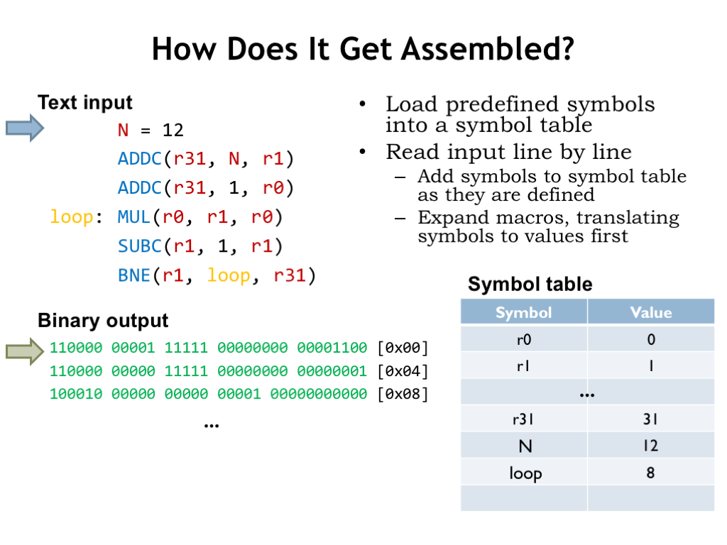
Let’s follow along as the assembler processes our source file. The assembler maintains a symbol table that maps symbols’ names to their numeric values. Initially the symbol table is loaded with mappings for all the register symbols.
The assembler reads the source file line-by-line, defining symbols and labels, expanding macros, or evaluating expressions to generate bytes for the output array. Whenever the assembler encounters a use of a symbol or label, it’s replaced by the corresponding numeric value found in the symbol table.
The first line, N = 12, defines the value of the symbol N to be 12, so the appropriate entry is made in the symbol table.
Advancing to the next line, the assembler encounters an invocation of the ADDC macro with the arguments “r31”, “N”, and “r1”. As we’ll see in a couple of slides, this triggers a series of nested macro expansions that eventually lead to generating a 32-bit binary value to be placed in memory location 0. The 32-bit value is formatted here to show the instruction fields and the destination address is shown in brackets.
The next instruction is processed in the same way, generating a second 32-bit word.
On the fourth line, the label loop is defined to have the value of the location in memory that’s about to filled (in this case, location 8). So the appropriate entry is made in the symbol table and the MUL macro is expanded into the 32-bit word to be placed in location 8.
The assembler processes the file line-by-line until it reaches the end of the file. Actually the assembler makes two passes through the file. On the first pass it loads the symbol table with the values from all the symbol and label definitions. Then, on the second pass, it generates the binary output. The two-pass approach allows a statement to refer to symbol or label that is defined later in the file, e.g., a forward branch instruction could refer to the label for an instruction later in the program.
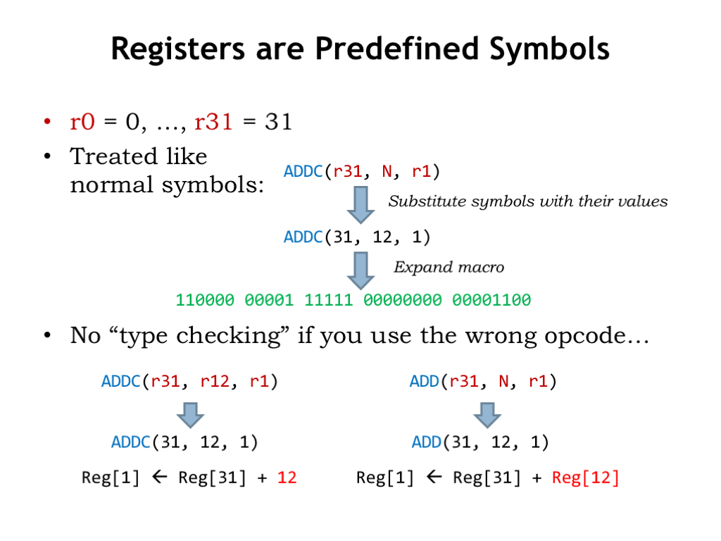
As we saw in the previous slide, there’s nothing magic about the register symbols — they are just symbolic names for the values 0 through 31. So when processing ADDC(r31,N,r1), UASM replaces the symbols with their values and actually expands ADDC(31,12,1).
UASM is very simple. It simply replaces symbols with their values, expands macros and evaluates expressions. So if you use a register symbol where a numeric value is expected, the value of the symbol is used as the numeric constant. Probably not what the programmer intended.
Similarly, if you use a symbol or expression where a register number is expected, the low-order 5 bits of the value is used as the register number, in this example, as the Rb register number. Again probably not what the programmer intended.
The moral of the story is that when writing UASM assembly language programs, you have to keep your wits about you and recognize that the interpretation of an operand is determined by the opcode macro, not by the way you wrote the operand.
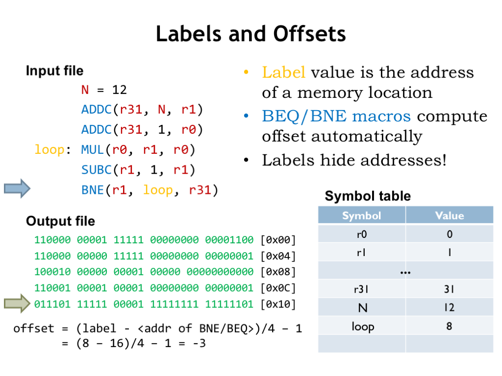
Recall from Lecture 9 that branch instructions use the 16-bit constant field of the instruction to encode the address of the branch target as a word offset from the location of the branch instruction. Well, actually the offset is calculated from the instruction immediately following the branch, so an offset of -1 would refer to the branch itself.
The calculation of the offset is a bit tedious to do by hand and would, of course, change if we added or removed instructions between the branch instruction and branch target. Happily macros for the branch instructions incorporate the necessary formula to compute the offset from the address of the branch and the address of the branch target. So we just specify the address of the branch target, usually with a label, and let UASM do the heavy lifting.
Here we see that BNE branches backwards by three instructions (remember to count from the instruction following the branch) so the offset is -3. The 16-bit two’s complement representation of -3 is the value placed in the constant field of the BNE instruction.
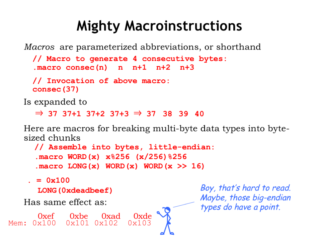
Let’s take a closer look at how macros work in UASM. Here we see the definition of the macro “consec” which has a single parameter “n”. The body of the macro is a sequence of four expressions. When there’s an invocation of the “consec” macro, in this example with the argument 37, the body of the macro is expanded replacing all occurrences of “n” with the argument 37. The resulting text is then processed as if it had appeared in place of the macro invocation. In this example, the four expressions are evaluated to give a sequence of four values that will be placed in the next four bytes of the output array.
Macro expansions may contain other macro invocations, which themselves will be expanded, continuing until all that’s left are expressions to be evaluated. Here we see the macro definition for WORD, which assembles its argument into two consecutive bytes. And for the macro LONG, which assembles its argument into four consecutive bytes, using the WORD macro to process the low 16 bits of the value, then the high 16 bits of the value.
These two UASM statements cause the constant 0xDEADBEEF to converted to 4 bytes, which are deposited in the output array starting at index 0x100.
Note that the Beta expects the least-significant byte of a multi-byte value to be stored at the lowest byte address. So the least-significant byte 0xEF is placed at address 0x100 and the most-significant byte 0xDE is placed at address 0x103. This is the “little-endian” convention for multi-byte values: the least-significant byte comes first. Intel’s x86 architecture is also little-endian.
There is a symmetrical “big-endian” convention where the most-significant byte comes first. Both conventions are in active use and, in fact, some ISAs can be configured to use either convention! There’s no “right answer” for which convention to use, but the fact that there two conventions means that we have to be alert for the need to convert the representation of multi-byte values when moving values between one ISA and another, e.g., when we send a data file to another user.
As you can imagine there are strong advocates for both schemes who are happy to defend their point of view at great length. Given the heat of the discussion, it’s appropriate that the names for the conventions were drawn from Jonathan Swift’s “Gulliver’s Travels” in which a civil war is fought over whether to open a soft-boiled egg at its big end or its little end.
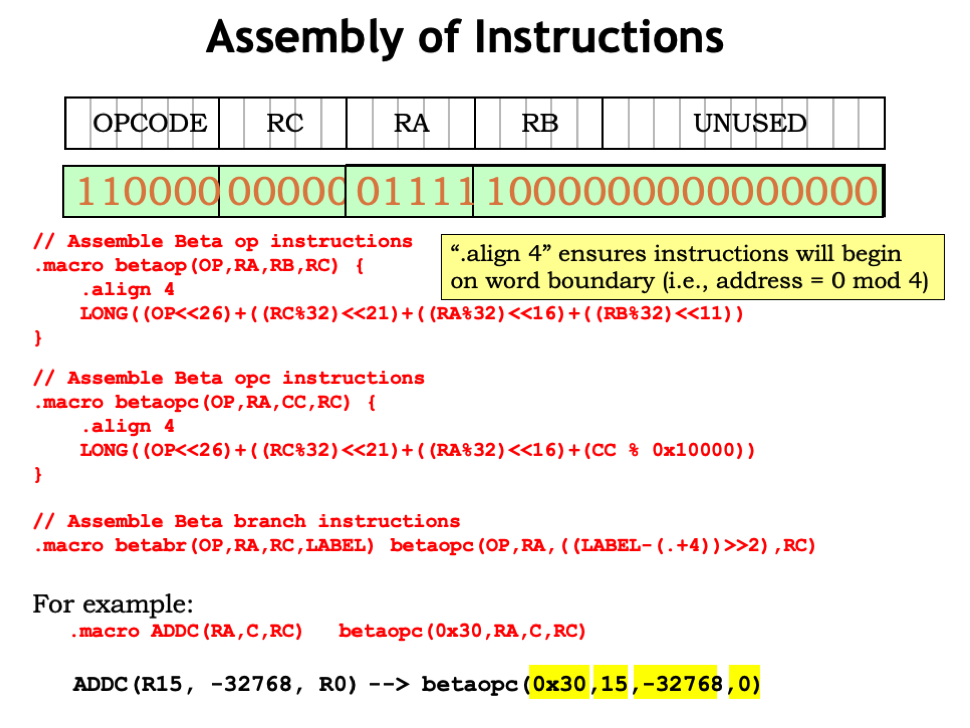
Let’s look at the macros used to assemble Beta instructions. The BETAOP helper macro supports the 3-register instruction format, taking as arguments the values to be placed in the OPCODE, Ra, Rb, and Rc fields. The “.align 4” directive is a bit of administrative bookkeeping to ensure that instructions will have a byte address that’s a multiple of 4, i.e., that they span exactly one 32-bit word in memory. That’s followed by an invocation of the LONG macro to generate the 4 bytes of binary data representing the value of the expression shown here. The expression is where the actual assembly of the fields takes place. Each field is limited to requisite number of bits using the modulo operator (%), then shifted left (<<) to the correct position in the 32-bit word.
And here are the helper macros for the instructions that use a 16-bit constant as the second operand.
Let’s follow the assembly of an ADDC instruction to see how this works. The ADDC macro expands into an invocation of the BETAOPC helper macro, passing along the correct value for the ADDC opcode, along with the three operands.
The BETAOPC macro does the following arithmetic: The OP argument, in this case the value 0x30, is shifted left to occupy the high-order 6 bits of the instruction. Then the RA argument, in this case 15, is placed in its proper location. The 16-bit constant -32768 is positioned in the low 16 bits of the instruction. And, finally, the Rc argument, in this case 0, is positioned in the Rc field of the instruction.
You can see why we call this processing “assembling an instruction”. The binary representation of an instruction is assembled from the binary values for each of the instruction fields. It’s not a complicated process, but it requires a lot of shifting and masking, tasks that we’re happy to let a computer handle.
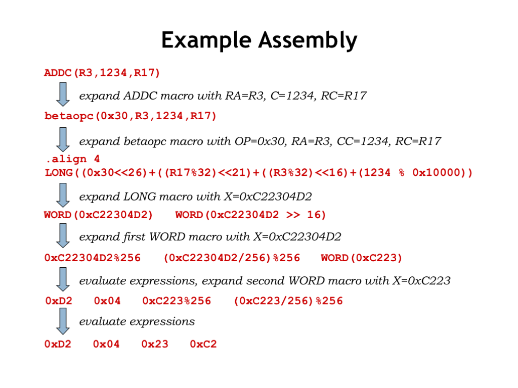
Here’s the entire sequence of macro expansions that assemble this ADDC instruction into an appropriate 32-bit binary value in main memory.
You can see that the knowledge of Beta instruction formats and opcode values is built into the bodies of the macro definitions. The UASM processing is actually quite general — with a different set of macro definitions it could process assembly language programs for almost any ISA!
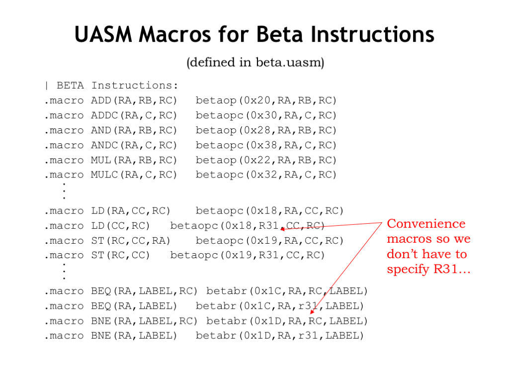
All the macro definitions for the Beta ISA are provided in the beta.uasm file, which is included in each of the assembly language lab assignments. Note that we include some convenience macros to define shorthand representations that provide common default values for certain operands. For example, except for procedure calls, we don’t care about the PC+4 value saved in the destination register by branch instructions, so almost always would specify R31 as the Rc register, effectively discarding the PC+4 value saved by branches. So we define two-argument branch macros that automatically provide R31 as the destination register. Saves some typing, and, more importantly, it makes it easier to understand the assembly language program.
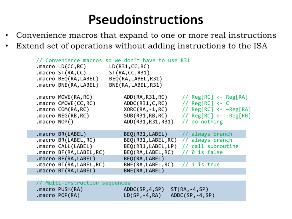
Here are a whole set of convenience macros intended to make programs more readable. For example, unconditional branches can be written using the BR() macro rather than the more cumbersome BEQ(R31,…). And it’s more readable to use branch-false (BF) and branch-true (BT) macros when testing the results of a compare instruction.
And note the PUSH and POP macros at the bottom of page. These expand into multi-instruction sequences, in this case to add and remove values from a stack data structure pointed to by the SP register.
We call these macros “pseudo instructions” since they let us provide the programmer with what appears a larger instruction set, although underneath the covers we’ve just using the same small instruction repertoire developed in Lecture 9.
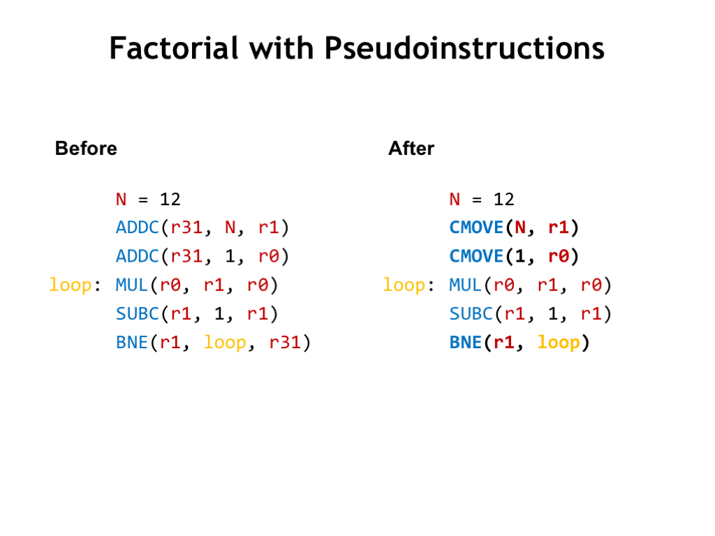
In this example we’ve rewritten the original code we had for the factorial computation using pseudo instructions. For example, CMOVE is a pseudo instruction for moving small constants into a register. It’s easier for us to read and understand the intent of a “constant move” operation than an “add a value to 0” operation provided by the ADDC expansion of CMOVE. Anything we can do to remove the cognitive clutter will be very beneficial in the long run.
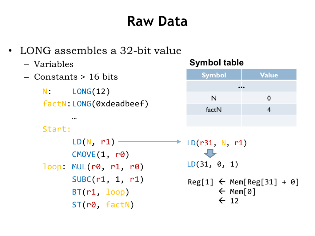
So far we’ve talked about assembling instructions. What about data? How do we allocate and initialize data storage and how do we get those values into registers so that they can be used as operands?
Here we see a program that allocates and initializes two memory locations using the LONG macro. We’ve used labels to remember the addresses of these locations for later reference.
When the program is assembled the values of the label N and factN are 0 and 4 respectively, the addresses of the memory locations holding the two data values.
To access the first data value, the program uses a LD instruction, in this case one of convenience macros that supplies R31 as the default value of the Ra field. The assembler replaces the reference to the label N with its value 0 from the symbol table. When the LD is executed, it computes the memory address by adding the constant (0) to the value of the Ra register (which is R31 and hence the value is 0) to get the address (0) of the memory location from which to fetch the value to be placed in R1.
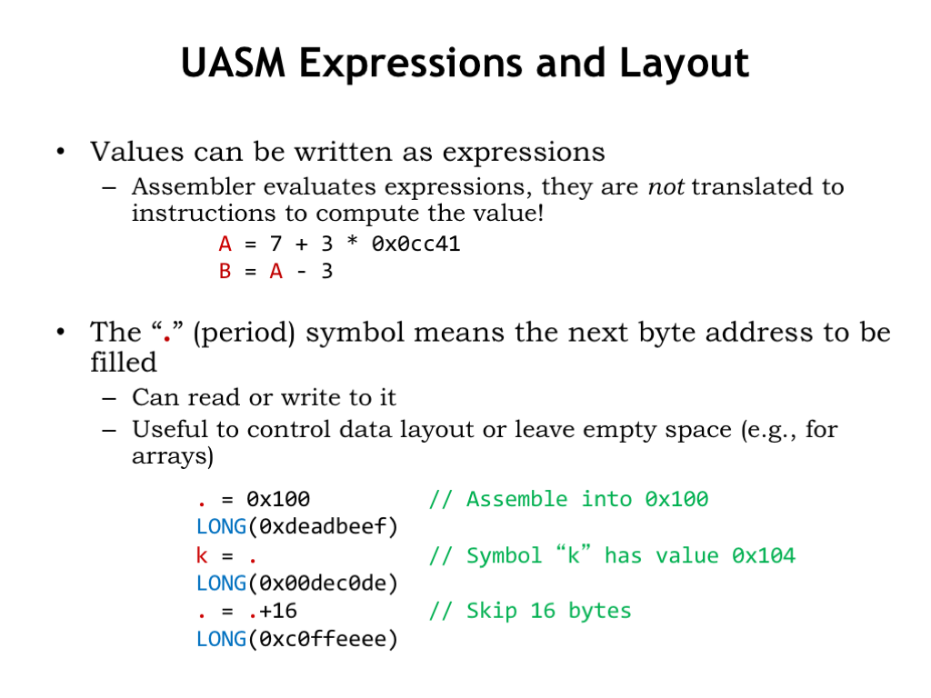
The constants needed as values for data words and instruction fields can be written as expressions. These expressions are evaluated by the assembler as it assembles the program and the resulting value is used as needed. Note that the expressions are evaluated at the time the assembler runs. By the time the program runs on the Beta, the resulting value is used. The assembler does NOT generate ADD and MUL instructions to compute the value during program execution. If a value is needed for an instruction field or initial data value, the assembler has to be able to perform the arithmetic itself. If you need the program to compute a value during execution, you have to write the necessary instructions as part of your program.
One last UASM feature: there’s a special symbol “.”, called “dot”, whose value is the address of the next main memory location to be filled by the assembler when it generates binary data. Initially “.” is 0 and it’s incremented each time a new byte value is generated.
We can set the value of “.” to tell the assembler where in memory we wish to place a value. In this example, the constant 0xDEADBEEF is placed into location 0x100 of main memory. And we can use “.” in expressions to compute the values for other symbols, as shown here when defining the value for the symbol “k”. In fact, the label definition “k:” is exactly equivalent to the UASM statement “k = .”
We can even increment the value of “.” to skip over locations, e.g., if we wanted to leave space for an un initialized array.
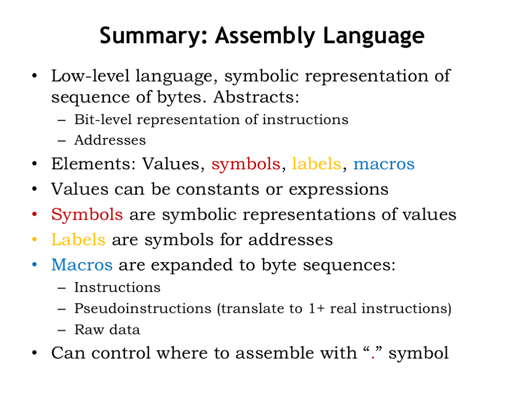
And that’s assembly language! We use assembly language as a convenient notation for generating the binary encoding for instructions and data. We let the assembler build the bit-level representations we need and to keep track of the addresses where these values are stored in main memory.
UASM itself provides support for values, symbols, labels and macros.
Values can be written as constants or expressions involving constants.
We use symbols to give meaningful names to values so that our programs will be more readable and more easily modified. Similarly, we use labels to give meaningful names to addresses in main memory and then use the labels in referring to data locations in LD or ST instructions, or to instruction locations in branch instructions.
Macros hide the details of how instructions are assembled from their component fields.
And we can use “.” to control where the assembler places values in main memory.
The assembler is itself a program that runs on our computer. That raises an interesting “chicken and egg problem”: how did the first assembler program get assembled into binary so it could run on a computer? Well, it was hand-assembled into binary. I suspect it processed a very simple language indeed, with the bells and whistles of symbols, labels, macros, expression evaluation, etc. added only after basic instructions could be assembled by the program. And I’m sure they were very careful not to lose the binary so they wouldn’t have to do the hand-assembly a second time!
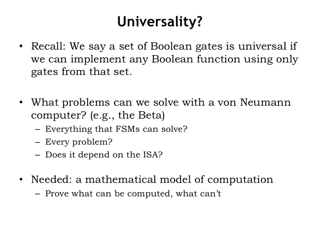
An interesting question for computer architects is what capabilities must be included in the ISA? When we studied Boolean gates in Part 1 of the course, we were able to prove that NAND were universal, i.e., that we could implement any Boolean function using only circuits constructed from NAND gates.
We can ask the corresponding question of our ISA: is it universal, i.e., can it be used to perform any computation? what problems can we solve with a von Neumann computer? Can the Beta solve any problem FSMs can solve? Are there problems FSMs can’t solve? If so, can the Beta solve those problems? Do the answers to these questions depend on the particular ISA?
To provide some answers, we need a mathematical model of computation. Reasoning about the model, we should be able to prove what can be computed and what can’t. And hopefully we can ensure that the Beta ISA has the functionality needed to perform any computation.
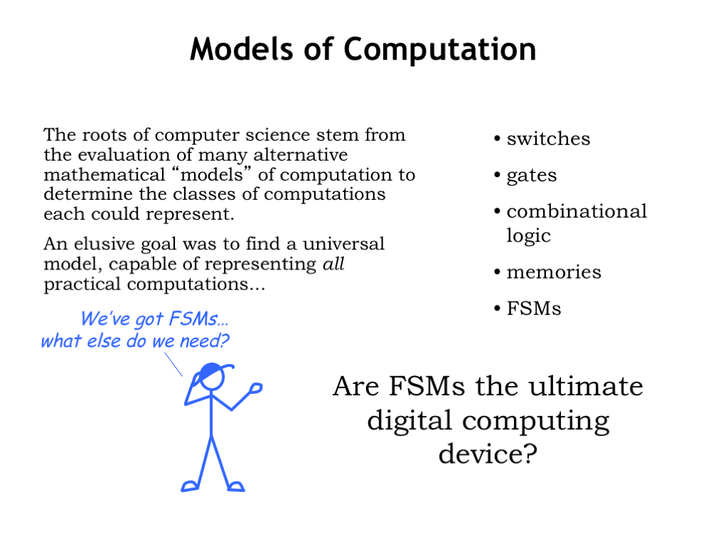
The roots of computer science stem from the evaluation of many alternative mathematical models of computation to determine the classes of computation each could represent. An elusive goal was to find a universal model, capable of representing *all* realizable computations. In other words if a computation could be described using some other well-formed model, we should also be able to describe the same computation using the universal model.
One candidate model might be finite state machines (FSMs), which can be built using sequential logic. Using Boolean logic and state transition diagrams we can reason about how an FSM will operate on any given input, predicting the output with 100% certainty.
Are FSMs the universal digital computing device? In other words, can we come up with FSM implementations that implement all computations that can be solved by any digital device?
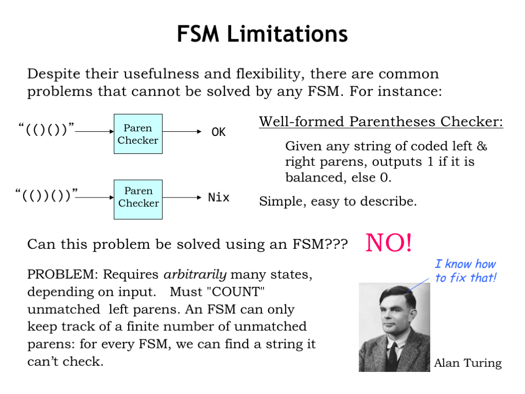
Despite their usefulness and flexibility, there are common problems that cannot be solved by any FSM. For example, can we build an FSM to determine if a string of parentheses (properly encoded into a binary sequence) is well-formed? A parenthesis string is well-formed if the parentheses balance, i.e., for every open parenthesis there is a matching close parenthesis later in the string. In the example shown here, the input string on the top is well-formed, but the input string on the bottom is not. After processing the input string, the FSM would output a 1 if the string is well-formed, 0 otherwise.
Can this problem be solved using an FSM? No, it can’t. The difficulty is that the FSM uses its internal state to encode what it knows about the history of the inputs. In the paren checker, the FSM would need to count the number of unbalanced open parens seen so far, so it can determine if future input contains the required number of close parens. But in a finite state machine there are only a fixed number of states, so a particular FSM has a maximum count it can reach. If we feed the FSM an input with more open parens than it has the states to count, it won’t be able to check if the input string is well-formed.
The “finite-ness” of FSMs limits their ability to solve problems that require unbounded counting. Hmm, what other models of computation might we consider? Mathematics to the rescue, in this case in the form of a British mathematician named Alan Turing.
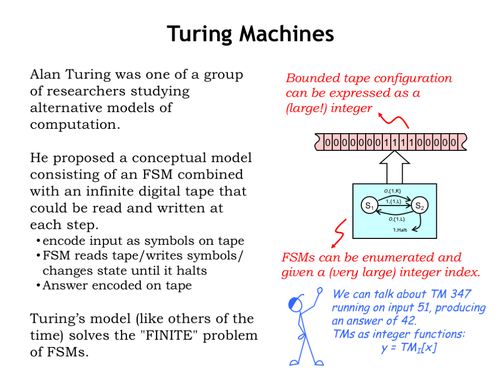
In the early 1930’s Alan Turing was one of many mathematicians studying the limits of proof and computation. He proposed a conceptual model consisting of an FSM combined with a infinite digital tape that could read and written under the control of the FSM. The inputs to some computation would be encoded as symbols on the tape, then the FSM would read the tape, changing its state as it performed the computation, then write the answer onto the tape and finally halting. Nowadays, this model is called a Turing Machine (TM). Turing Machines, like other models of the time, solved the “finite” problem of FSMs.
So how does all this relate to computation? Assuming the non-blank input on the tape occupies a finite number of adjacent cells, it can be expressed as a large integer. Just construct a binary number using the bit encoding of the symbols from the tape, alternating between symbols to the left of the tape head and symbols to the right of the tape head. Eventually all the symbols will be incorporated into the (very large) integer representation.
So both the input and output of the TM can be thought of as large integers, and the TM itself as implementing an integer function that maps input integers to output integers.
The FSM brain of the Turing Machine can be characterized by its truth table. And we can systematically enumerate all the possible FSM truth tables, assigning an index to each truth table as it appears in the enumeration. Note that indices get very large very quickly since they essentially incorporate all the information in the truth table. Fortunately we have a very large supply of integers!
We’ll use the index for a TM’s FSM to identify the TM as well. So we can talk about TM 347 running on input 51, producing the answer 42.
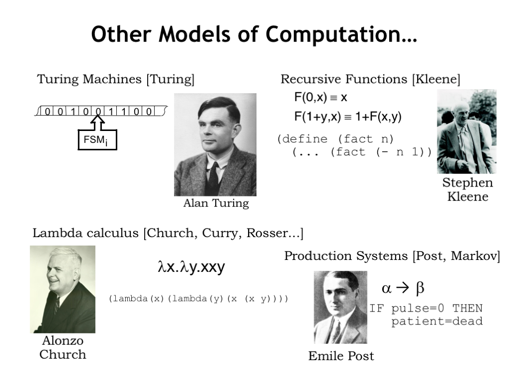
There are many other models of computation, each of which describes a class of integer functions where a computation is performed on an integer input to produce an integer answer. Kleene, Post and Turing were all students of Alonzo Church at Princeton University in the mid-1930’s. They explored many other formulations for modeling computation: recursive functions, rule-based systems for string rewriting, and the lambda calculus. They were all particularly intrigued with proving the existence of problems unsolvable by realizable machines. Which, of course, meant characterizing the problems that could be solved by realizable machines.
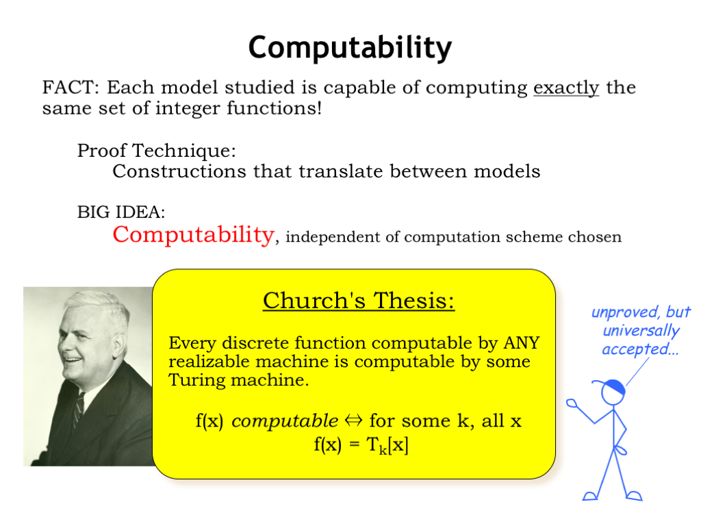
It turned out that each model was capable of computing exactly the same set of integer functions! This was proved by coming up with constructions that translated the steps in a computation between the various models. It was possible to show that if a computation could be described by one model, an equivalent description exists in the other model. This lead to a notion of computability that was independent of the computation scheme chosen. This notion is formalized by Church’s Thesis, which says that every discrete function computable by any realizable machine is computable by some Turing Machine. So if we say the function f(x) is computable, that’s equivalent to saying that there’s a TM that given x as an input on its tape will write f(x) as an output on the tape and halt.
As yet there’s no proof of Church’s Thesis, but it’s universally accepted that it’s true. In general “computable” is taken to mean “computable by some TM”.
If you’re curious about the existence of uncomputable functions, please see the optional video at the end of this lecture.
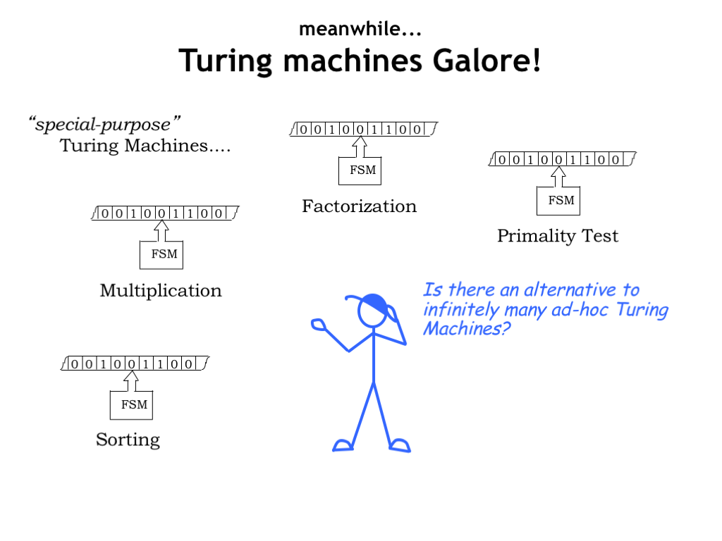
Okay, we’ve decided that Turing Machines can model any realizable computation. In other words for every computation we want to perform, there’s a (different) Turing Machine that will do the job. But how does this help us design a general-purpose computer? Or are there some computations that will require a special-purpose machine no matter what?
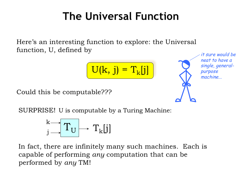
What we’d like to find is a universal function U: it would take two arguments, k and j, and then compute the result of running \(T_k\) on input j. Is U computable, i.e., is there a universal Turing Machine \(T_U\)? If so, then instead of many ad-hoc TMs, we could just use \(T_U\) to compute the results for any computable function.
Surprise! U is computable and \(T_U\) exists. If fact there are infinitely many universal TMs, some quite simple - the smallest known universal TM has 4 states and uses 6 tape symbols. A universal machine is capable of performing any computation that can be performed by any TM!
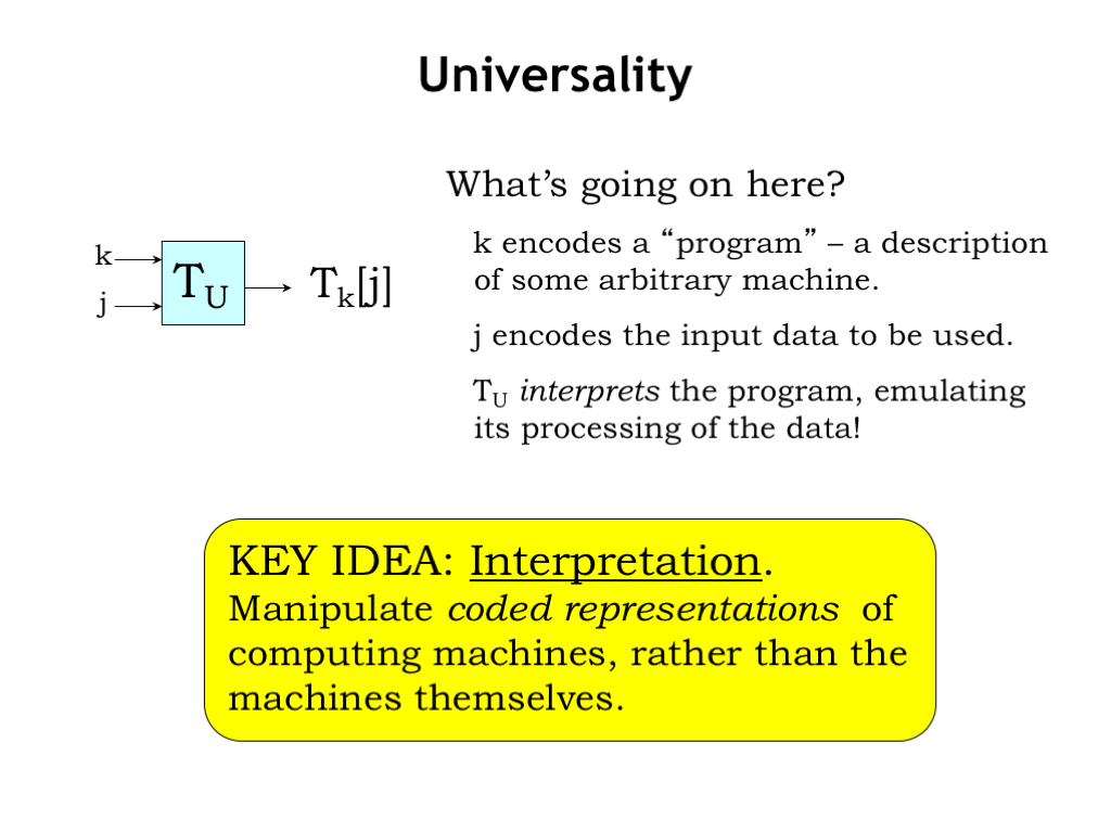
What’s going on here? k encodes a “program” - a description of some arbitrary TM that performs a particular computation. j encodes the input data on which to perform that computation. \(T_U\) “interprets” the program, emulating the steps \(T_k\) will take to process the input and write out the answer. The notion of interpreting a coded representation of a computation is a key idea and forms the basis for our stored program computer.
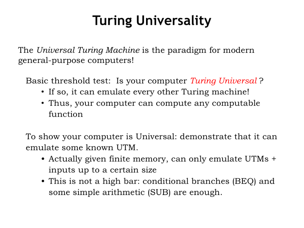
The Universal Turing Machine is the paradigm for modern general-purpose computers. Given an ISA we want to know if it’s equivalent to a universal Turing Machine. If so, it can emulate every other TM and hence compute any computable function.
How do we show our computer is Turing Universal? Simply demonstrate that it can emulate some known Universal Turing Machine. The finite memory on actual computers will mean we can only emulate UTM operations on inputs up to a certain size, but within this limitation we can show our computer can perform any computation that fits into memory.
As it turns out this is not a high bar: so long as the ISA has conditional branches and some simple arithmetic, it will be Turing Universal.
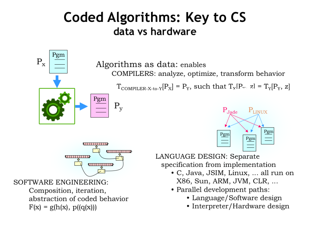
This notion of encoding a program in a way that allows it to be data to some other program is a key idea in computer science.
We often translate a program Px written to run on some abstract high-level machine (eg, a program in C or Java) into, say, an assembly language program Py that can be interpreted by our CPU. This translation is called compilation.
Much of software engineering is based on the idea of taking a program and using it as as component in some larger program.
Given a strategy for compiling programs, that opens the door to designing new programming languages that let us express our desired computation using data structures and operations particularly suited to the task at hand.
So what have we learned from the mathematicians’ work on models of computation? Well, it’s nice to know that the computing engine we’re planning to build will be able to perform any computation that can be performed on any realizable machine. And the development of the universal Turing Machine model paved the way for modern stored-program computers. The bottom line: we’re good to go with the Beta ISA!
We’ve discussed computable functions. Are there uncomputable functions?
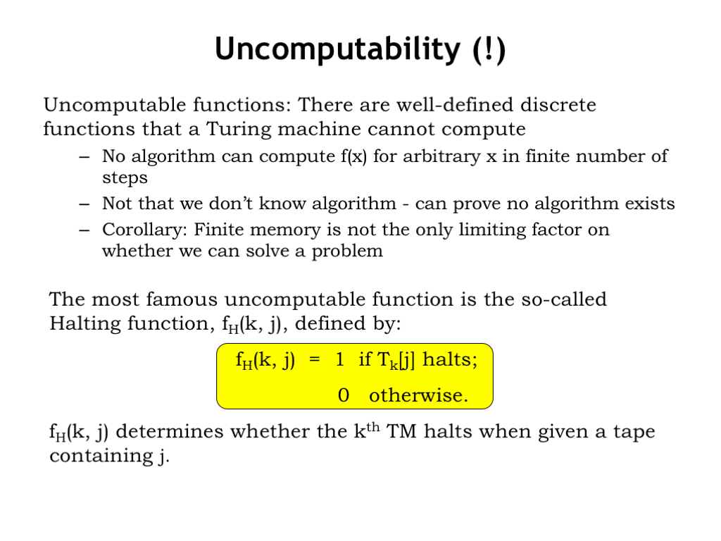
Yes, there are well-defined discrete functions that cannot be computed by any TM, i.e., no algorithm can compute f(x) for arbitrary finite x in a finite number of steps. It’s not that we don’t know the algorithm, we can actually prove that no algorithm exists. So the finite memory limitation of FSMs wasn’t the only barrier as to whether we can solve a problem.
The most famous uncomputable function is the so-called Halting function. When TMs undertake a computation there two possible outcomes. Either the TM writes an answer onto the tape and halts, or the TM loops forever. The Halting function tells which outcome we’ll get: given two integer arguments k and j, the Halting function determines if the kth TM halts when given a tape containing j as the input.
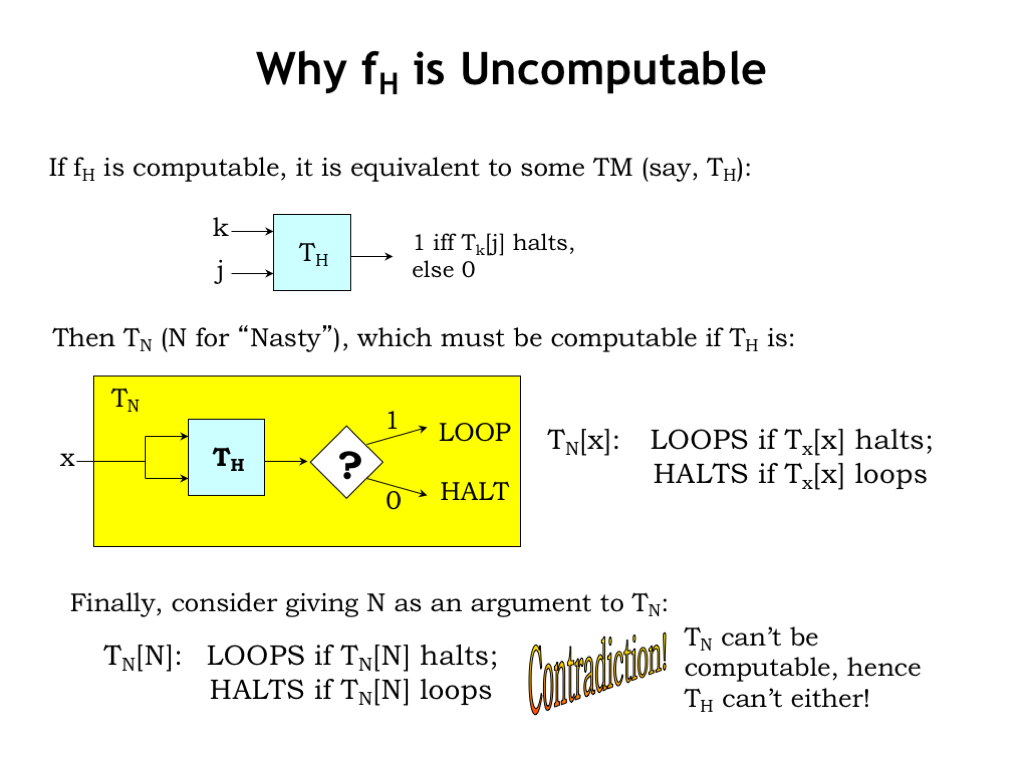
Let’s quickly sketch an argument as to why the Halting function is not computable. Well, suppose it was computable, then it would be equivalent to some TM, say \(T_H\).
So we can use \(T_H\) to build another TM, \(T_N\) (the “N” stands for nasty!) that processes its single argument and either LOOPs or HALTs. \(T_N[X]\) is designed to loop if TM X given input X halts. And vice versa: \(T_N[X]\) halts if TM X given input X loops. The idea is that \(T_N[X]\) does the opposite of whatever \(T_X[X]\) does. \(T_N\) is easy to implement assuming that we have \(T_H\) to answer the “halts or loops” question.
Now consider what happens if we give N as the argument to \(T_N\). From the definition of \(T_N\), \(T_N[N]\) will LOOP if the halting function tells us that \(T_N[N]\) halts. And \(T_N[N]\) will HALT if the halting function tells us that \(T_N[N]\) loops. Obviously \(T_N[N]\) can’t both LOOP and HALT at the same time! So if the Halting function is computable and \(T_H\) exists, we arrive at this impossible behavior for \(T_N[N]\). This tells us that \(T_H\) cannot exist and hence that the Halting function is not computable.


