
L12: Procedures and Stacks
- Procedures: A Software Abstraction
- Implementing Procedures
- Procedure Calling Convention
- Procedure Linkage: First Try
- Procedure Storage Needs
- Activation Records
- Insight: We Need a Stack!
- Stack Implementation
- Stack Management Macros
- Fun With Stacks
- Solving Procedure Linkage Problems
- Stack Frames as Activation Records
- Stack Frame Details
- Argument Order & BP Usage
- Procedure Linkage: The Contract
- Procedure Linkage Templates
- Putting It All Together: Factorial
- Recursion?
- Stack Detective
- Summary of Dedicated Registers
- Summary
Content of the following slides is described in the surrounding text.
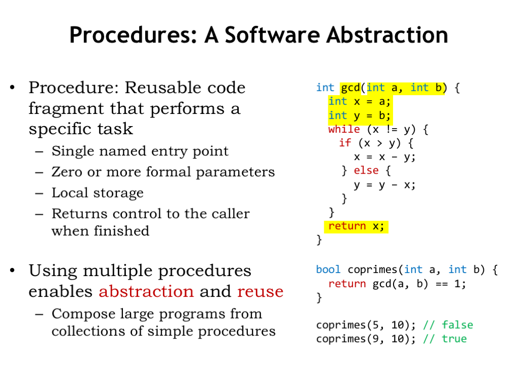
One of the most useful abstractions provided by high-level languages is the notion of a procedure or subroutine, which is a sequence of instructions that perform a specific task.
A procedure has a single named entry point, which can be used to refer to the procedure in other parts of the program. In the example here, this code is defining the GCD procedure, which is declared to return an integer value.
Procedures have zero or more formal parameters, which are the names the code inside the procedure will use to refer the values supplied when the procedure is invoked by a “procedure call”. A procedure call is an expression that has the name of the procedure followed by parenthesized list of values called “arguments” that will be matched up with the formal parameters. For example, the value of the first argument will become the value of the first formal parameter while the procedure is executing.
The body of the procedure may define additional variables, called “local variables”, since they can only be accessed by statements in the procedure body. Conceptually, the storage for local variables only exists while the procedure is executing. They are allocated when the procedure is invoked and deallocated when the procedure returns.
The procedure may return a value that’s the result of the procedure’s computation. It’s legal to have procedures that do not return a value, in which case the procedures would only be executed for their “side effects”, e.g., changes they make to shared data.
Here we see another procedure, COPRIMES, that invokes the GCD procedure to compute the greatest common divisor of two numbers. To use GCD, the programmer of COPRIMES only needed to know the input/output behavior of GCD, i.e., the number and types of the arguments and what type of value is returned as a result. The procedural abstraction has hidden the implementation of GCD, while still making its functionality available as a “black box”.
This is a very powerful idea: encapsulating a complex computation so that it can be used by others. Every high-level language comes with a collection of pre-built procedures, called “libraries”, which can be used to perform arithmetic functions (e.g., square root or cosine), manipulate collections of data (e.g., lists or dictionaries), read data from files, and so on — the list is nearly endless! Much of the expressive power and ease-of-use provided by high-level languages comes from their libraries of “black boxes”.
The procedural abstraction is at the heart of object-oriented languages, which encapsulate data and procedures as black boxes called objects that support specific operations on their internal data. For example, a LIST object has procedures (called “methods” in this context) for indexing into the list to read or change a value, adding new elements to the list, inquiring about the length of the list, and so on. The internal representation of the data and the algorithms used to implement the methods are hidden by the object abstraction. Indeed, there may be several different LIST implementations to choose from depending on which operations you need to be particularly efficient.
Okay, enough about the virtues of the procedural abstraction! Let’s turn our attention to how to implement procedures using the Beta ISA.
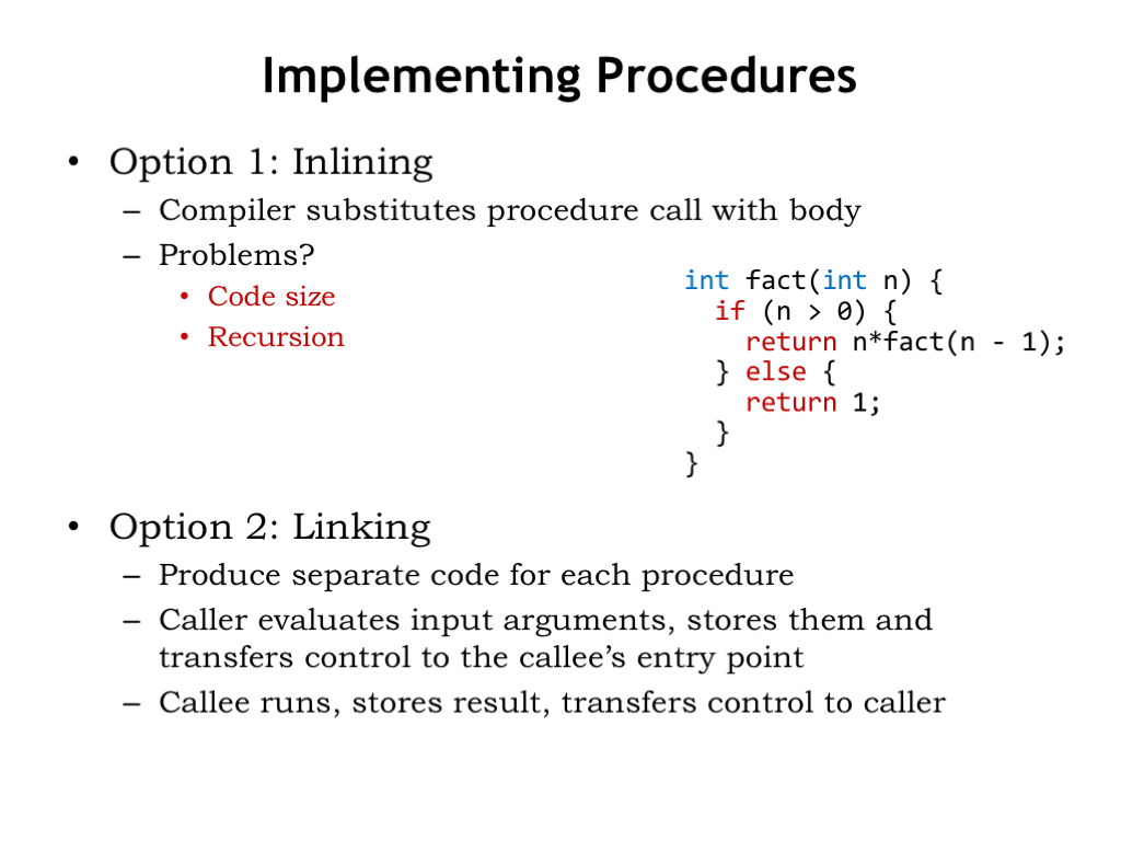
A possible implementation is to “inline” the procedure, where we replace the procedure call with a copy of the statements in the procedure’s body, substituting argument values for references to the formal parameters. In this approach we’re treating procedures very much like UASM macros, i.e., a simple notational shorthand for making a copy of the procedure’s body.
Are there any problems with this approach? One obvious issue is the potential increase in the code size. For example, if we had a lengthy procedure that was called many times, the final expanded code would be huge! Enough so that inlining isn’t a practical solution except in the case of short procedures where optimizing compilers do sometimes decide to inline the code.
A bigger difficulty is apparent when we consider a recursive procedure where there’s a nested call to the procedure itself. During execution the recursion will terminate for some values of the arguments and the recursive procedure will eventually return an answer. But at compile time, the inlining process would not terminate and so the inlining scheme fails if the language allows recursion.
The second option is to “link” to the procedure. In this approach there is a single copy of the procedure code which we arrange to be run for each procedure call — all the procedure calls are said to link to the procedure code.
Here the body of the procedure is translated once into Beta instructions and the first instruction is identified as the procedure’s entry point. The procedure call is compiled into a set of instructions that evaluate the argument expressions and save the values in an agreed-upon location. Then we’ll use a BR instruction to transfer control to the entry point of the procedure. Recall that the BR instruction not only changes the PC but saves the address of the instruction following the branch in a specified register. This saved address is the “return address” where we want execution to resume when procedure execution is complete.
After branching to the entry point, the procedure code runs, stores the result in an agreed-upon location and then resumes execution of the calling program by jumping to the supplied return address.
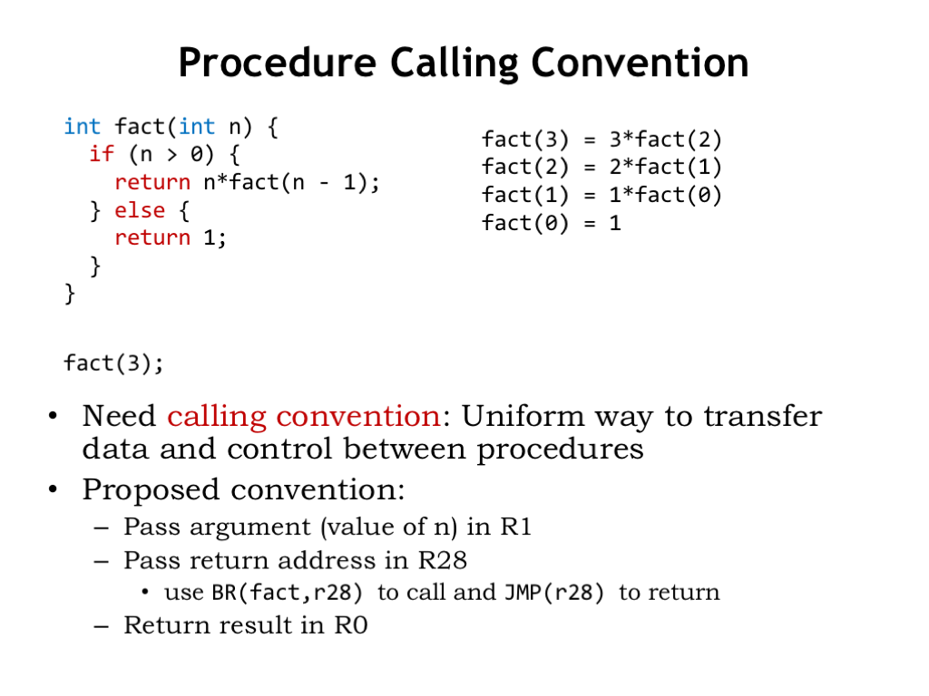
To complete this implementation plan we need a “calling convention” that specifies where to store the argument values during procedure calls and where the procedure should store the return value. It’s tempting to simply allocate specific memory locations for the job: how about using registers? We could pass the argument value in registers starting, say, with R1. The return address could be stored in another register, say R28. As we can see, with this convention the BR and JMP instructions are just what we need to implement procedure call and return. It’s usual to call the register holding the return address the “linkage pointer”. And finally the procedure can use, say, R0 to hold the return value.
Let’s see how this would work when executing the procedure call fact(3). As shown on the right, fact(3) requires a recursive call to compute fact(2), and so on. Our goal is to have a uniform calling convention where all procedure calls and procedure bodies use the same convention for storing arguments, return addresses and return values. In particular, we’ll use the same convention when compiling the recursive call fact(n-1) as we did for the initial call to fact(3).
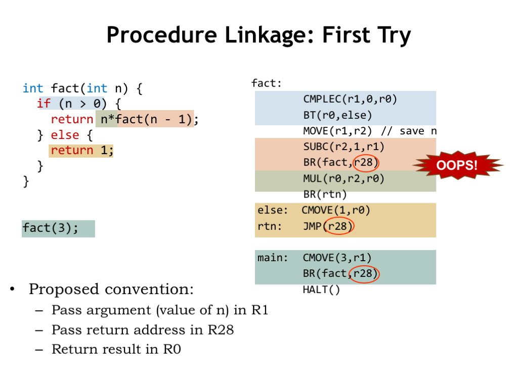
Okay. In the code shown on the right we’ve used our proposed convention when compiling the Beta code for fact(). Let’s take a quick tour.
To compile the initial call fact(3) the compiler generated a CMOVE instruction to put the argument value in R1 and then a BR instruction to transfer control to fact’s entry point while remembering the return address in R28.
The first statement in the body of fact tests the value of the argument using CMPLEC and BT instructions.
When n is greater than 0, the code performs a recursive call to fact, saving the value of the recursive argument n-1 in R1 as our convention requires. Note that we had to first save the value of the original argument n because we’ll need it for the multiplication after the recursive call returns its value in R0.
If n is not greater than 0, the value 1 is placed in R0. Then the two possible execution paths merge, each having generated the appropriate return value in R0, and finally there’s a JMP to return control to the caller. The JMP instruction knows to find the return address in R28, just where the BR put it as part of the original procedure call.
Some of you may have noticed that there are some difficulties with this particular implementation. The code is correct in the sense that it faithfully implements procedure call and return using our proposed convention. The problem is that during recursive calls we’ll be overwriting register values we need later.
For example, note that following our calling convention, the recursive call also uses R28 to store the return address. When executed, the code for the original call stored the address of the HALT instruction in R28. Inside the procedure, the recursive call will store the address of the MUL instruction in R28. Unfortunately that overwrites the original return address.
Even the attempt to save the value of the argument N in R2 is doomed to fail since during the execution of the recursive call R2 will be overwritten.
The crux of the problem is that each recursive call needs to remember the value of its argument and return address, i.e., we need two storage locations for each active call to fact(). And while executing fact(3), when we finally get to calling fact(0) there are four nested active calls, so we’ll need 4*2 = 8 storage locations. In fact, the amount of storage needed varies with the depth of the recursion. Obviously we can’t use just two registers (R2 and R28) to hold all the values we need to save.
One fix is to disallow recursion! And, in fact, some of the early programming languages such as FORTRAN did just that. But let’s see if we can solve the problem another way.
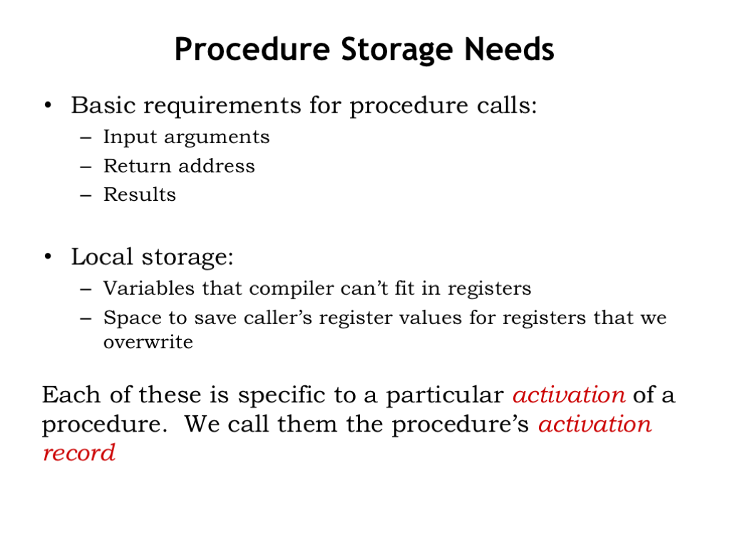
The problem we need to solve is where to store the values needed by procedure: its arguments, its return address, its return value. The procedure may also need storage for its local variables and space to save the values of the caller’s registers before they get overwritten by the procedure. We’d like to avoid any limitations on the number of arguments, the number of local variables, etc.
So we’ll need a block of storage for each active procedure call, what we’ll call the “activation record”. As we saw in the factorial example, we can’t statically allocate a single block of storage for a particular procedure since recursive calls mean we’ll have many active calls to that procedure at points during the execution.
What we need is a way to dynamically allocate storage for an activation record when the procedure is called, which can then be reclaimed when the procedure returns.
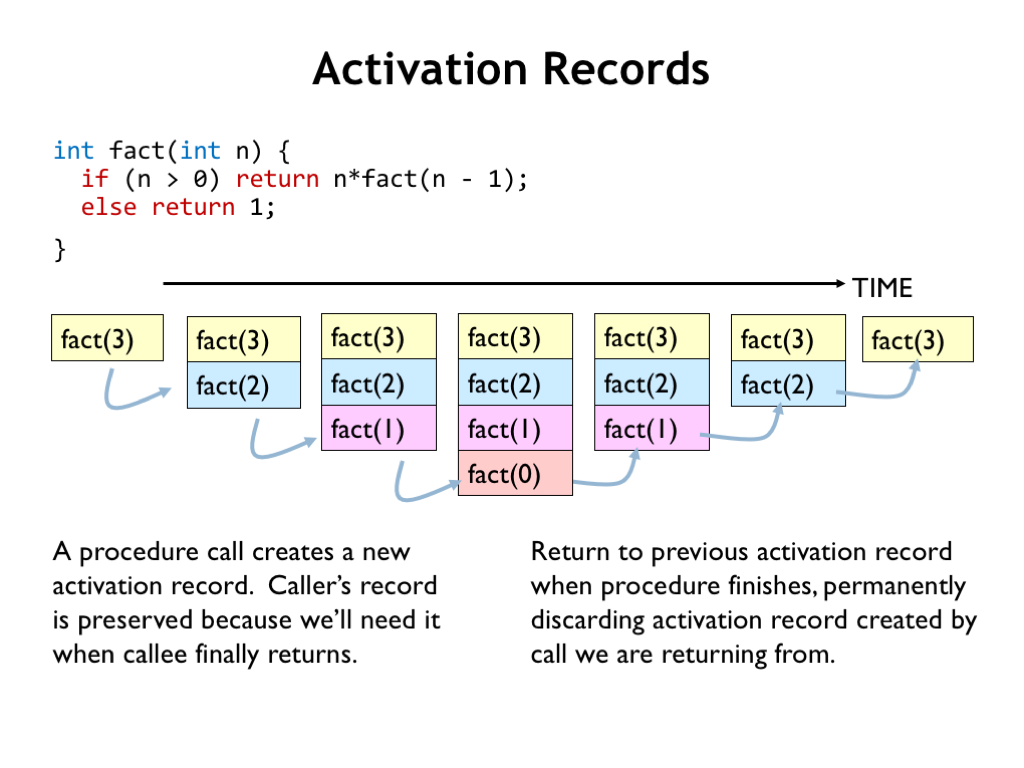
Let’s see how activation records come and go as execution proceeds.
The first activation record is for the call fact(3). It’s created at the beginning of the procedure and holds, among other things, the value of the argument n and the return address where execution should resume after the fact(3) computation is complete.
During the execution of fact(3), we need to make a recursive call to compute fact(2). So that procedure call also gets an activation record with the appropriate values for the argument and return address. Note that the original activation record is kept since it contains information needed to complete the computation of fact(3) after the call to fact(2) returns. So now we have two active procedure calls and hence two activation records.
fact(2) requires computing fact(1), which, in turn, requires computing fact(0). At this point there are four active procedure calls and hence four activation records.
The recursion terminates with fact(0), which returns the value 1 to its caller. At this point we’ve finished execution of fact(0) and so its activation record is no longer needed and can be discarded.
fact(1) now finishes its computation returning 1 to its caller. We no longer need its activation record. Then fact(2) completes, returning 2 to its caller and its activation can be discarded. And so on…
Note that the activation record of a nested procedure call is always discarded before the activation record of the caller. That makes sense: the execution of the caller can’t complete until the nested procedure call returns. What we need is a storage scheme that efficiently supports the allocation and deallocation of activation records as shown here.
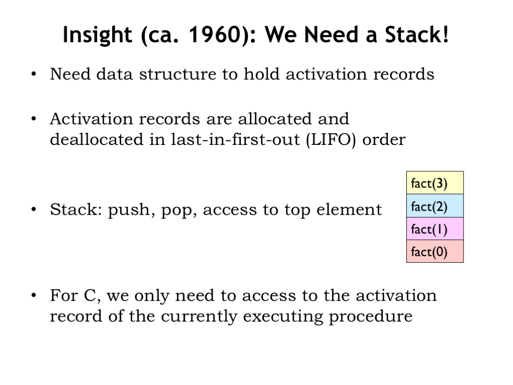
Early compiler writers recognized that activation records are allocated and deallocated in last-in first-out (LIFO) order. So they invented the “stack”, a data structure that implements a PUSH operation to add a record to the top of the stack and a POP operation to remove the top element. New activation records are PUSHed onto the stack during procedure calls and the POPed from the stack when the procedure call returns. Note that stack operations affect the top (i.e., most recent) record on the stack.
C procedures only need to access the top activation record on the stack. Other programming languages, e.g. Java, support accesses to other active activation records. The stack supports both modes of operation.
One final technical note: some programming languages support closures (e.g., Javascript) or continuations (e.g., Python’s yield statement), where the activation records need to be preserved even after the procedure returns. In these cases, the simple LIFO behavior of the stack is no longer sufficient and we’ll need another scheme for allocating and deallocating activation records. But that’s a topic for another course!

Here’s how we’ll implement the stack on the Beta:
We’ll dedicate one of the Beta registers, R29, to be the “stack pointer” that will be used to manage stack operations.
When we PUSH a word onto the stack, we’ll increment the stack pointer. So the stack grows to successively higher addresses as words are PUSHed onto the stack.
We’ll adopt the convention that SP points to (i.e., its value is the address of) the first unused stack location, the location that will be filled by next PUSH. So locations with addresses lower than the value in SP correspond to words that have been previously allocated.
Words can be PUSHed to or POPed from the stack at any point in execution, but we’ll impose the rule that code sequences that PUSH words onto the stack must POP those words at the end of execution. So when a code sequence finishes execution, SP will have the same value as it had before the sequence started. This is called the “stack discipline” and ensures that intervening uses of the stack don’t affect later stack references.
We’ll allocate a large region of memory to hold the stack located so that the stack can grow without overwriting other program storage. Most systems require that you specify a maximum stack size when running a program and will signal an execution error if the program attempts to PUSH too many items onto the stack.
For our Beta stack implementation, we’ll use existing instructions to implement stack operations, so for us the stack is strictly a set of software conventions. Other ISAs provide instructions specifically for stack operations.
There are many other sensible stack conventions, so you’ll need to read up on the conventions adopted by the particular ISA or programming language you’ll be using.
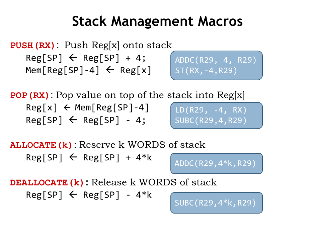
We’ve added some convenience macros to UASM to support stacks.
The PUSH macro expands into two instructions. The ADDC increments the stack pointer, allocating a new word at the top of stack, and then initializes the new top-of-stack from a specified register value with a ST instruction.
The POP macro LDs the value at the top of the stack into the specified register, then uses a SUBC instruction to decrement the stack pointer, deallocating that word from the stack.
Note that the order of the instructions in the PUSH and POP macro is very important. As we’ll see in the next lecture, interrupts can cause the Beta hardware to stop executing the current program between any two instructions, so we have to be careful about the order of operations. So for PUSH, we first allocate the word on the stack, then initialize it. If we did it the other way around and execution was interrupted between the initialization and allocation, code run during the interrupt which uses the stack might unintentionally overwrite the initialized value. But, assuming all code follows stack discipline, allocation followed by initialization is always safe.
The same reasoning applies to the order of the POP instructions. We first access the top-of-stack one last time to retrieve its value, then we deallocate that location.
We can use the ALLOCATE macro to reserve a number of stack locations for later use. Sort of like PUSH but without the initialization.
DEALLOCATE performs the opposite operation, removing N words from the stack.
In general, if we see a PUSH or ALLOCATE in an assembly language program, we should be able to find the corresponding POP or DEALLOCATE, which would indicate that stack discipline is maintained.
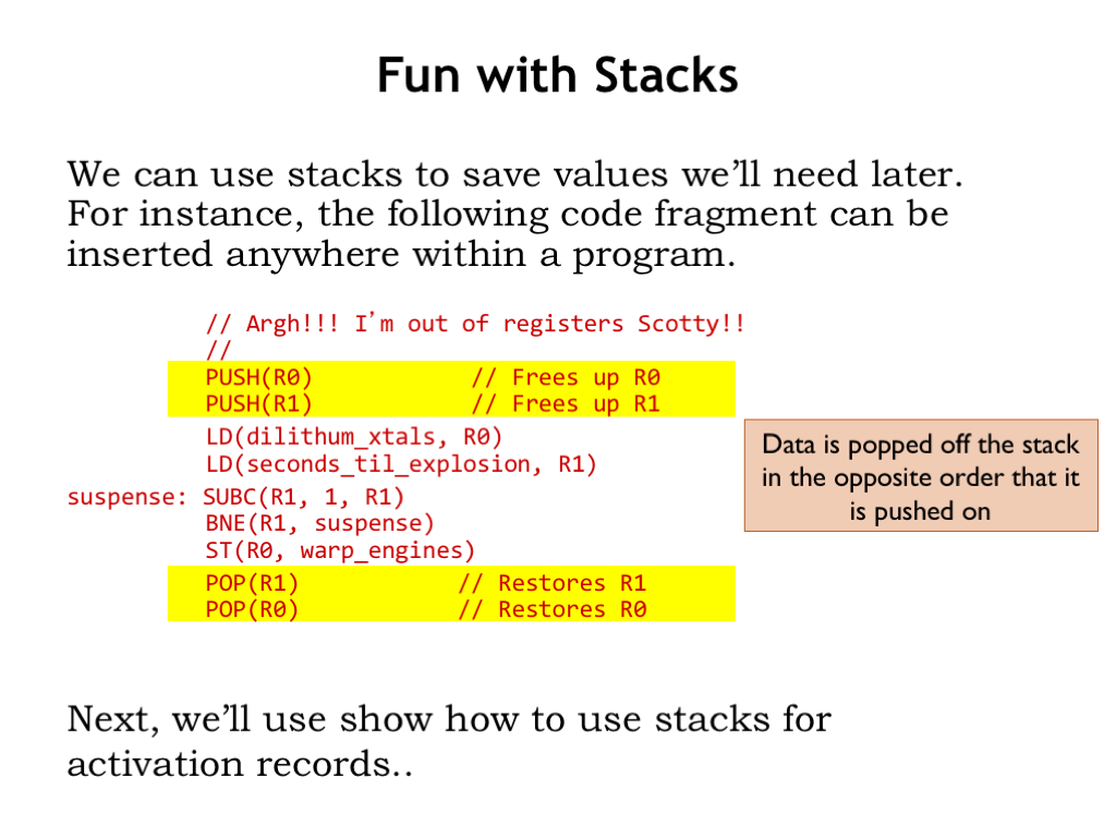
We’ll use stacks to save values we’ll need later. For example, if we need to use some registers for a computation but don’t know if the register’s current values are needed later in the program, we can PUSH their current values onto the stack and then are free to use the registers in our code. After we’re done, we can use POP to restore the saved values.
Note that we POP data off the stack in the opposite order that the data was PUSHed, i.e., we need to follow the last-in first-out discipline imposed by the stack operations.
Now that we have the stack data structure, we’ll use it to solve our problems with allocating and deallocating activation records during procedure calls.
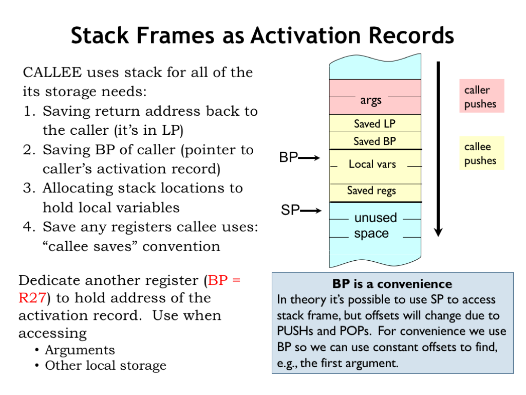
We’ll use the stack to hold a procedure’s activation record. That includes the values of the arguments to the procedure call. We’ll allocate words on the stack to hold the values of the procedure’s local variables, assuming we don’t keep them in registers. And we’ll use the stack to save the return address (passed in LP) so the procedure can make nested procedure calls without overwriting its return address.
The responsibility for allocating and deallocating the activation record will be shared between the calling procedure (the “caller”) and the called procedure (the “callee”).
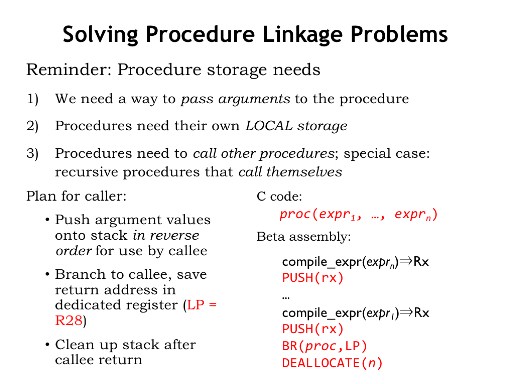
The caller is responsible for evaluating the argument expressions and saving their values in the activation record being built on the stack. We’ll adopt the convention that argument values are pushed in reverse order, i.e., the first argument will be the last to be pushed on the stack. We’ll explain why we made this choice in a couple of slides…
The code compiled for a procedure involves a sequence of expression evaluations, each followed by a PUSH to save the calculated value on the stack. So when the callee starts execution, the top of the stack contains the value of the first argument, the next word down the value of the second argument, and so on.
After the argument values, if any, have been pushed on the stack, there’s a BR to transfer control to the procedure’s entry point, saving the address of the instruction following the BR in the linkage pointer, R28, a register that we’ll dedicate to that task.
When the callee returns and execution resumes in the caller, a DEALLOCATE is used to remove all the argument values from the stack, preserving stack discipline.
So that’s the code the compiler generates for the procedure. The rest of the work happens in the called procedure.
The code at the start of the called procedure completes the allocation of the activation record. Since when we’re done the activation record will occupy a bunch of consecutive words on the stack, we’ll sometimes refer to the activation record as a “stack frame” to remind us of where it lives.
The first action is to save the return address found in the LP register. This frees up LP to be used by any nested procedure calls in the body of the callee.
In order to make it easy to access values stored in the activation record, we’ll dedicate another register called the “base pointer” (BP = R27) which will point to the stack frame we’re building. So as we enter the procedure, the code saves the pointer to the caller’s stack frame, and then uses the current value of the stack pointer to make BP point to the current stack frame. We’ll see how we use BP in just a moment.
Now the code will allocate words in the stack frame to hold the values for the callee’s local variables, if any.
Finally, the callee needs to save the values of any registers it will use when executing the rest of its code. These saved values can be used to restore the register values just before returning to the caller. This is called the “callee saves” convention where the callee guarantees that all register values will be preserved across the procedure call. With this convention, the code in the caller can assume any values it placed in registers before a nested procedure call will still be there when the nested call returns.
Note that dedicating a register as the base pointer isn’t strictly necessary. All accesses to the values on the stack can be made relative to the stack pointer, but the offsets from SP will change as values are PUSHed and POPed from the stack, e.g., during procedure calls. It will be easier to understand the generated code if we use BP for all stack frame references.
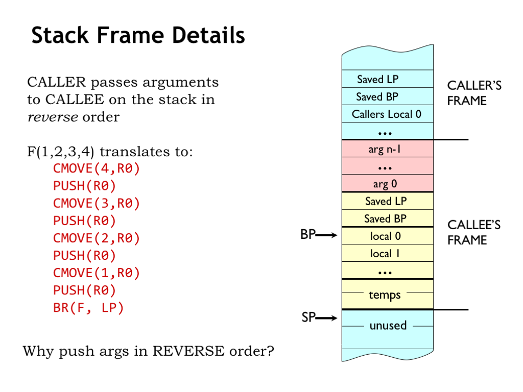
Let’s return to the question about the order of argument values in the stack frame. We adopted the convention of PUSHing the values in reverse order, i.e., where the value of the first argument is the last one to be PUSHED.
So, why PUSH argument values in reverse order?

With the arguments PUSHed in reverse order, the first argument (labeled “arg 0”) will be at a fixed offset from the base pointer regardless of the number of argument values pushed on the stack. The compiler can use a simple formula to the determine the correct BP offset value for any particular argument. So the first argument is at offset -12, the second at -16, and so on.
Why is this important? Some languages, such as C, support procedure calls with a variable number of arguments. Usually the procedure can determine from, say, the first argument, how many additional arguments to expect. The canonical example is the C printf function where the first argument is a format string that specifies how a sequence of values should be printed. So a call to printf includes the format string argument plus a varying number of additional arguments. With our calling convention the format string will always be in the same location relative to BP, so the printf code can find it without knowing the number of additional arguments in the current call.
The local variables are also at fixed offsets from BP. The first local variable is at offset 0, the second at offset 4, and so on.
So we see that having a base pointer makes it easy to access the values of the arguments and local variables using fixed offsets that can be determined at compile time. The stack above the local variables is available for other uses, e.g., building the activation record for a nested procedure call!
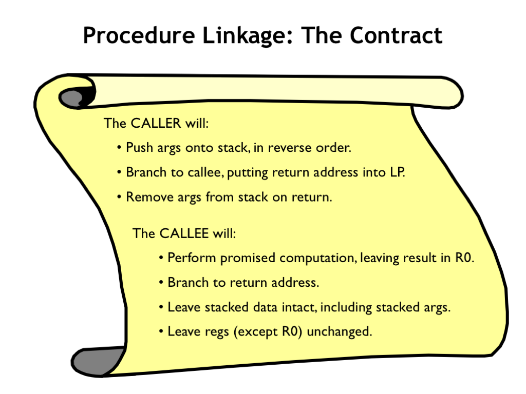
Okay, here’s our final contract for how procedure calls will work:
The calling procedure (“caller”) will
PUSH the argument values onto the stack in reverse order.
Branch to the entry point of the callee, putting the return address into the linkage pointer.
When the callee returns, remove the argument values from the stack.
The called procedure (“callee”) will
Perform the promised computation, leaving the result in R0.
Jump to the return address when the computation has finished.
Remove any items it has placed on the stack, leaving the stack as it was when the procedure was entered. Note that the arguments were PUSHed on the stack by the caller, so it will be up to the caller to remove them.
Preserve the values in all registers except R0, which holds the return value. So the caller can assume any values placed in registers before a nested call will be there when the nested call returns.

We saw the code template for procedure calls on an earlier slide.
Here’s the template for the entry point to a procedure F. The code saves the caller’s LP and BP values, initializes BP for the current stack frame and allocates words on the stack to hold any local variable values. The final step is to PUSH the value of any registers (besides R0) that will be used by the remainder of the procedure’s code.
The template for the exit sequence mirrors the actions of the entry sequence, restoring all the values saved by the entry sequence, performing the POP operations in the reverse of the order of the PUSH operations in the entry sequence. Note that in moving the BP value into SP we’ve reset the stack to its state at the point of the MOVE(SP,BP) in the entry sequence. This implicitly undoes the effect of the ALLOCATE statement in the entry sequence, so we don’t need a matching DEALLOCATE in the exit sequence.
The last instruction in the exit sequence transfers control back to the calling procedure.
With practice you’ll become familiar with these code templates. Meanwhile, you can refer back to this slide whenever you need to generate code for a procedure call.

Here’s the code our compiler would generate for the C implementation of factorial shown on the left.
The entry sequence saves the caller’s LP and BP, then initializes BP for the current stack frame. The value of R1 is saved so we can use R1 in code that follows.
The exit sequence restores all the saved values, including that for R1. The code for the body of the procedure has arranged for R0 to contain the return value by the time execution reaches the exit sequence.
The nested procedure call passes the argument value on the stack and removes it after the nested call returns.
The remainder of the code is generated using the templates we saw in the previous lecture. Aside from computing and pushing the values of the arguments, there are approximately 10 instructions needed to implement the linking approach to a procedure call. That’s not much for a procedure of any size, but might be significant for a trivial procedure. As mentioned earlier, some optimizing compilers can make the tradeoff of inlining small non-recursive procedures saving this small amount of overhead.
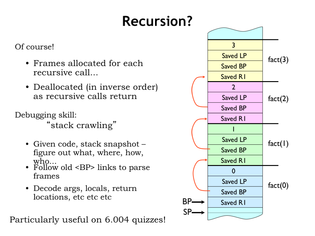
So have we solved the activation record storage issue for recursive procedures?
Yes! A new stack frame is allocated for each procedure call. In each frame we see the storage for the argument and return address [CLICK]. And as the nested calls return the stack frames will be deallocated in inverse order.
Interestingly we can learn a lot about the current state of execution by looking at the active stack frames. The current value of BP, along with the older values saved in the activation records, allow us to identify the active procedure calls and determine their arguments, the values of any local variables for active calls, and so on. If we print out all this information at any given time we would have a “stack trace” showing the progress of the computation. In fact, when a problem occurs, many language runtimes will print out the stack trace to help the programmer determine what happened.
And, of course, if you can interpret the information in the stack frames, you can show you understand our conventions for procedure call and return. Don’t be surprised to find such a question on a quiz :)
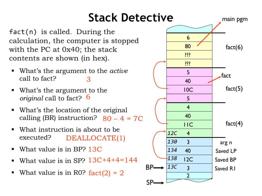
Let’s practice our newfound skill and see what we can determine about a running program which we’ve stopped somewhere in the middle of its execution. We’re told that a computation of fact() is in progress and that the PC of the next instruction to be executed is 0x40. We’re also given the stack dump shown on right.
Since we’re in the middle of a fact computation, we know that current stack frame (and possibly others) is an activation record for the fact function. Using the code on the previous slide we can determine the layout of the stack frame and generate the annotations shown on the right of the stack dump. With the annotations, it’s easy to see that the argument to current active call is the value 3.
Now we want to know the argument to original call to fact. We’ll have to label the other stack frames using the saved BP values. Looking at the saved LP values for each frame (always found at an offset of -8 from the frame’s BP), we see that many of the saved values are 0x40, which must be the return address for the recursive fact calls.
Looking through the stack frames we find the first return address that’s *not* 0x40, which must an return address to code that’s not part of the fact procedure. This means we’ve found the stack frame created by the original call to fact and can see that argument to the original call is 6.
What’s the location of the BR that made the original call? Well the saved LP in the stack frame of the original call to fact is 0x80. That’s the address of the instruction following the original call, so the BR that made the original call is one instruction earlier, at location 0x7C. To answer these questions you have to be good at hex arithmetic!
What instruction is about to be executed? We were told its address is 0x40, which we notice is the saved LP value for all the recursive fact calls. So 0x40 must be the address of the instruction following the BR(fact,LP) instruction in the fact code. Looking back a few slides at the fact code, we see that’s a DEALLOCATE(1) instruction.
What value is in BP? Hmm. We know BP is the address of the stack location containing the saved R1 value in the current stack frame. So the saved BP value in the current stack frame is the address of the saved R1 value in the *previous* stack frame. So the saved BP value gives us the address of a particular stack location, from which we can derive the address of all the other locations! Counting forward, we find that the value in BP must be 0x13C.
What value is in SP? Since we’re about to execute the DEALLOCATE to remove the argument of the nested call from the stack, that argument must still be on the stack right after the saved R1 value. Since the SP points to first unused stack location, it points to the location after that word, so it has the value 0x144.
Finally, what value is is R0? Since we’ve just returned from a call to fact(2) the value in R0 must the result from that recursive call, which is 2.
Wow! You can learn a lot from the stacked activation records and a little deduction! Since the state of the computation is represented by the values of the PC, the registers, and main memory, once we’re given that information we can tell exactly what the program has been up to. Pretty neat…
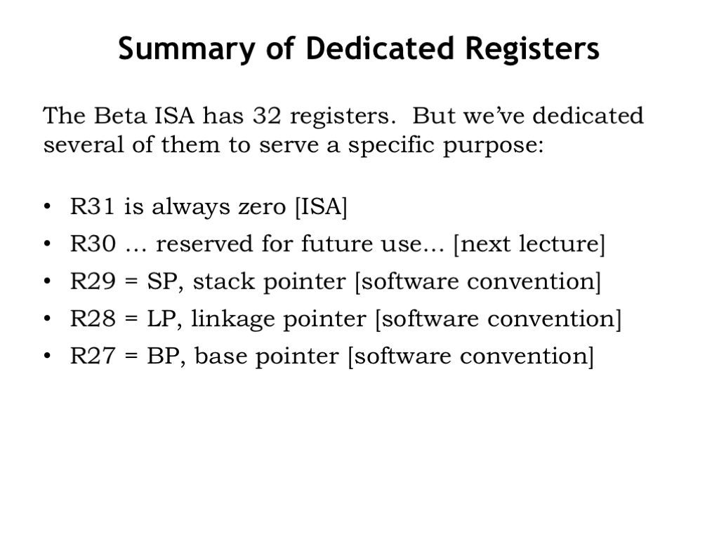
Wrapping up, we’ve been dedicating some registers to help with our various software conventions. To summarize:
R31 is always zero, as defined by the ISA.
We’ll also dedicate R30 to a particular function in the ISA when we discuss the implementation of the Beta in the next lecture. Meanwhile, don’t use R30 in your code!
The remaining dedicated registers are connected with our software conventions:
R29 (SP) is used as the stack pointer,
R28 (LP) is used as the linkage pointer, and
R27 (BP) is used as the base pointer.
As you practice reading and writing code, you’ll grow familiar with these dedicated registers.
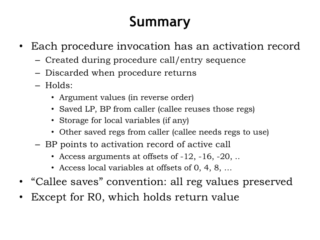
In thinking about how to implement procedures, we discovered the need for an activation record to store the information needed by any active procedure call.
An activation record is created by the caller and callee at the start of a procedure call. And the record can be discarded when the procedure is complete.
The activation records hold argument values, saved LP and BP values along with the caller’s values in any other of the registers. Storage for the procedure’s local variables is also allocated in the activation record.
We use BP to point to the current activation record, giving easy access to the values of the arguments and local variables.
We adopted a “callee saves” convention where the called procedure is obligated to preserve the values in all registers except for R0.
Taken together, these conventions allow us to have procedures with arbitrary numbers of arguments and local variables, with nested and recursive procedure calls. We’re now ready to compile and execute any C program!


