
.toc { margin-left: 2em; } .lecslide { margin-top: 1em; margin-bottom: 1em; border-top: 0.5px solid #808080; padding-top: 1em; text-align: center; } .lecslideimg { width: 5in; border: 1px solid black; }
- Reminder: Single-Cycle Beta
- Single-Cycle Beta Performance
- Pipelined Implementation
- Why Isn’t This a 20-Minute Lecture?
- Pipeline Hazards
- Simplified Unpipelined Beta Datapath
- 5-Stage Pipelined Datapath
- Pipelined Control
- Pipelined Execution Example
- Example: Cycle 1
- Example: Cycle 2
- Example: Cycle 3
- Example: Cycle 4
- Example: Cycle 5
- Pipeline Diagrams
- Data Hazards
- Resolving Hazards I
- Resolving Data Hazards I
- Stall Logic
- Resolving Data Hazards II
- Bypass Logic
- Fully Bypassed Pipeline
- Load-to-Use Stalls
- Summary: Pipelining with Data Hazards
- Compilers Can Help
- Or Take the Lazy Route…
- Control Hazards I
- Control Hazards II
- Resolving Control Hazards
- Resolving Control Hazards with Stalls
- Stall Logic for Control Hazards
- ISA Issues: Simple vs. Complex Branches
- Resolving Hazards II
- Resolving Hazards with Speculation I
- Resolving Hazards with Speculation II
- Speculation Logic For Control Hazards
- Branch Prediction
- Branch Delay Slots I
- Branch Delay Slots II
- Exceptions
- When Can Exceptions Happen?
- Resolving Exceptions
- Exception Handling Logic
- Multiple Exceptions?
- Asynchronous Interrupts
- Exception + Interrupt Handling Logic
- 5-Stage Beta: Final Version
- Reminder: Resolving Hazards
Content of the following slides is described in the surrounding text.
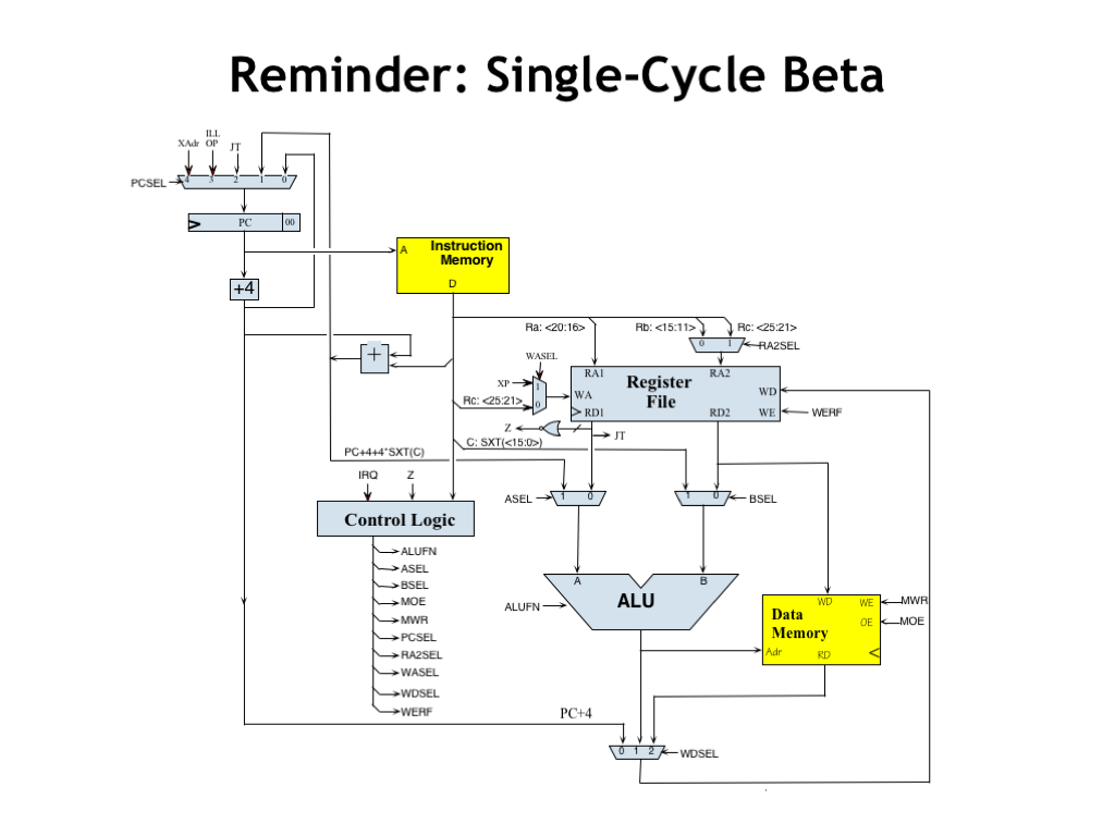
In this lecture, we’re going to use the circuit pipelining techniques we learned earlier in the course to improve the performance of the 32-bit Beta CPU design we developed earlier in the course. This CPU design executes one Beta instruction per clock cycle. Hopefully you remember the design! If not, you might find it worthwhile to review “Building the Beta”.
At the beginning of the clock cycle, this circuit loads a new value into the program counter, which is then sent to main memory as the address of the instruction to be executed this cycle. When the 32-bit word containing the binary encoding of the instruction is returned by the memory, the opcode field is decoded by the control logic to determine the control signals for the rest of the data path. The operands are read from the register file and routed to the ALU to perform the desired operation. For memory operations, the output of the ALU serves as the memory address and, in the case of load instructions, the main memory supplies the data to be written into the register file at the end of the cycle. PC+4 and ALU values can also be written to the register file.
The clock period of the Beta is determined by the cumulative delay through all the components involved in instruction execution. Today’s question is: how can we make this faster?
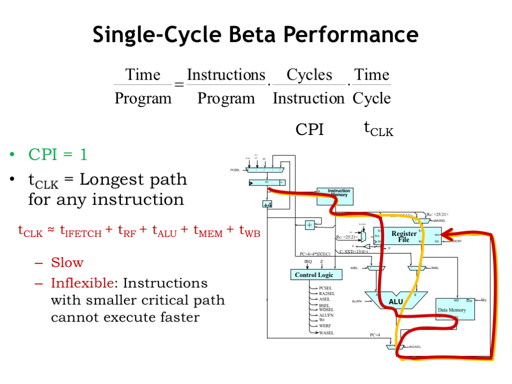
We can characterize the time spent executing a program as the product of three terms. The first term is the total number of instructions executed. Since the program usually contains loops and procedure calls, many of the encoded instructions will be executed many times. We want the total count of instructions executed, not the static size of the program as measured by the number of encoded instructions in memory. The second term is the average number of clock cycles it takes to execute a single instruction. And the third term is the duration of a single clock cycle.
As CPU designers it’s the last two terms which are under our control: the cycles per instruction (CPI) and the clock period (\(t_{\textrm{CLK}}\)). To affect the first term, we would need to change the ISA or write a better compiler!
Our design for the Beta was able to execute every instruction in a single clock cycle, so our CPI is 1. As we discussed in the previous slide, \(t_{\textrm{CLK}}\) is determined by the longest path through the Beta circuitry. For example, consider the execution of an OP-class instruction, which involves two register operands and an ALU operation. The arrow shows all the components that are involved in the execution of the instruction. Aside from a few MUXes, the main memory, register file, and ALU must all have time to do their thing.
The worst-case execution time is for the LD instruction. In one clock cycle we need to fetch the instruction from main memory (\(t_{\textrm{IFETCH}}\)), read the operands from the register file (\(t_{\textrm{RF}}\)), perform the address addition in the ALU (\(t_{\textrm{ALU}}\)), read the requested location from main memory (\(t_{\textrm{MEM}}\)), and finally write the memory data to the destination register (\(t_{\textrm{WB}}\)).
The component delays add up and the result is a fairly long clock period and hence it will take a long time to run the program. And our two example execution paths illustrate another issue: we’re forced to choose the clock period to accommodate the worst-case execution time, even though we may be able to execute some instructions faster since their execution path through the circuitry is shorter. We’re making all the instructions slower just because there’s one instruction that has a long critical path.
So why not have simple instructions execute in one clock cycle and more complex instructions take multiple cycles instead of forcing all instructions to execute in a single, long clock cycle? As we’ll see in the next few slides, we have a good answer to this question, one that will allow us to execute *all* instructions with a short clock period.
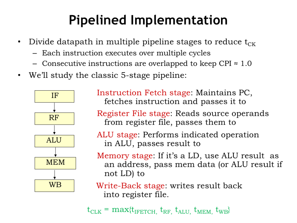
We’re going to use pipelining to address these issues. We’re going to divide the execution of an instruction into a sequence of steps, where each step is performed in successive stages of the pipeline. So it will take multiple clock cycles to execute an instruction as it travels through the stages of the execution pipeline. But since there are only one or two components in each stage of the pipeline, the clock period can be much shorter and the throughput of the CPU can be much higher.
The increased throughput is the result of overlapping the execution of consecutive instructions. At any given time, there will be multiple instructions in the CPU, each at a different stage of its execution. The time to execute all the steps for a particular instruction (i.e., the instruction latency) may be somewhat higher than in our unpipelined implementation. But we will finish the last step of executing some instruction in each clock cycle, so the instruction throughput is 1 per clock cycle. And since the clock cycle of our pipelined CPU is quite a bit shorter, the instruction throughput is quite a bit higher.
All this sounds great, but, not surprisingly, there are few issues we’ll have to deal with.
There are many ways to pipeline the execution of an instruction. We’re going to look at the design of the classic 5-stage instruction execution pipeline, which was widely used in the integrated circuit CPU designs of the 1980’s.
The 5 pipeline stages correspond to the steps of executing an instruction in a von-Neumann stored-program architecture. The first stage (IF) is responsible for fetching the binary-encoded instruction from the main memory location indicated by the program counter.
The 32-bit instruction is passed to the register file stage (RF) where the required register operands are read from the register file.
The operand values are passed to the ALU stage (ALU), which performs the requested operation.
The memory stage (MEM) performs the second access to main memory to read or write the data for LD, LDR, or ST instructions, using the value from the ALU stage as the memory address. For load instructions, the output of the MEM stage is the read data from main memory. For all other instructions, the output of the MEM stage is simply the value from the ALU stage.
In the final write-back stage (WB), the result from the earlier stages is written to the destination register in the register file.
Looking at the execution path from the previous slide, we see that each of the main components of the unpipelined design is now in its own pipeline stage. So the clock period will now be determined by the slowest of these components.
Having divided instruction execution into five stages, would we expect the clock period to be one fifth of its original value? Well, that would only happen if we were able to divide the execution so that each stage performed exactly one fifth of the total work. In real life, the major components have somewhat different latencies, so the improvement in instruction throughput will be a little less than the factor of 5 a perfect 5-stage pipeline could achieve. If we have a slow component, e.g., the ALU, we might choose to pipeline that component into further stages, or, interleave multiple ALUs to achieve the same effect. But for this lecture, we’ll go with the 5-stage pipeline described above.
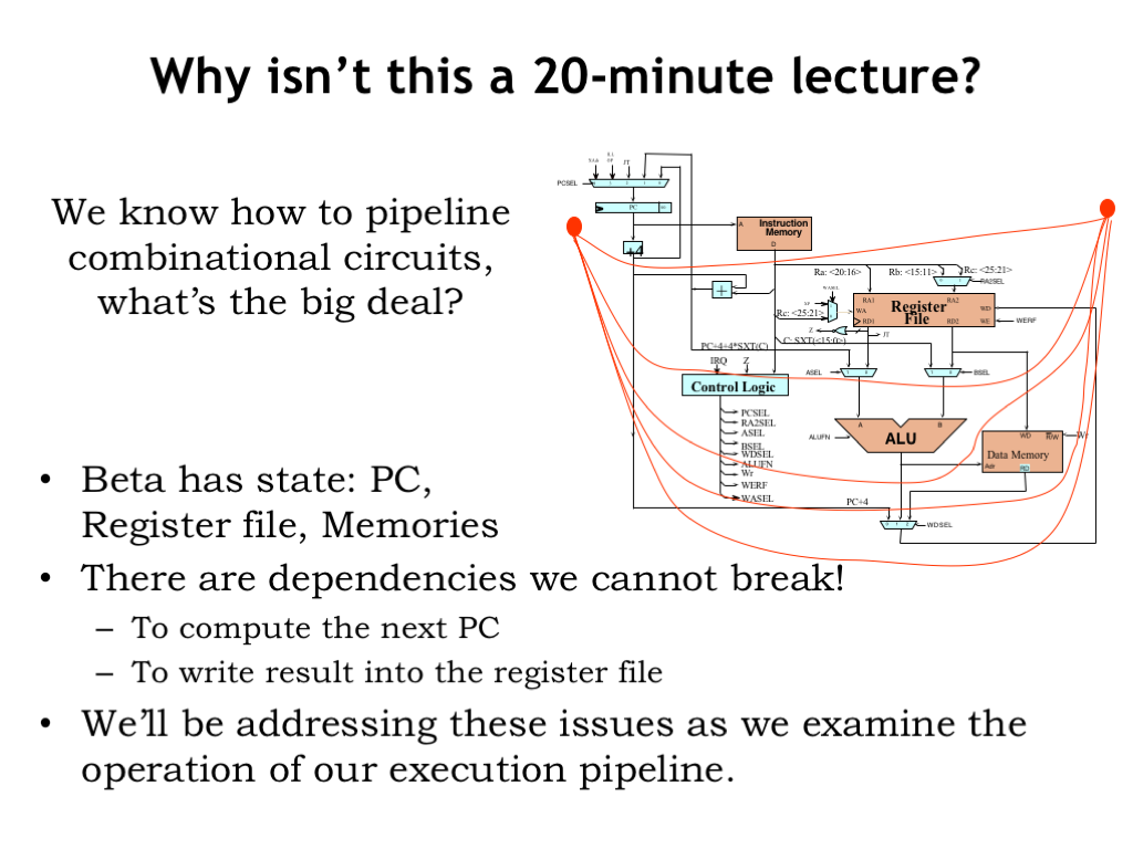
So why isn’t this a 20-minute lecture? After all we know how pipeline combinational circuits: we can build a valid k-stage pipeline by drawing k contours across the circuit diagram and adding a pipeline register wherever a contour crosses a signal. What’s the big deal here?
Well, is this circuit combinational? No! There’s state in the registers and memories. This means that the result of executing a given instruction may depend on the results from earlier instructions. There are loops in the circuit where data from later pipeline stages affects the execution of earlier pipeline stages. For example, the write to the register file at the end of the WB stage will change values read from the register file in the RF stage. In other words, there are execution dependencies between instructions and these dependencies will need to be taken into account when we’re trying to pipeline instruction execution. We’ll be addressing these issues as we examine the operation of our execution pipeline.

Sometimes execution of a given instruction will depend on the results of executing a previous instruction. Two are two types of problematic dependencies.
The first, termed a data hazard, occurs when the execution of the current instruction depends on data produced by an earlier instruction. For example, an instruction that reads R0 will depend on the execution of an earlier instruction that wrote R0.
The second, termed a control hazard, occurs when a branch, jump, or exception changes the order of execution. For example, the choice of which instruction to execute after a BNE depends on whether the branch is taken or not.
Instruction execution triggers a hazard when the instruction on which it depends is also in the pipeline, i.e., the earlier instruction hasn’t finished execution! We’ll need to adjust execution in our pipeline to avoid these hazards.
Here’s our plan of attack:
We’ll start by designing a 5-stage pipeline that works with sequences of instructions that don’t trigger hazards, i.e., where instruction execution doesn’t depend on earlier instructions still in the pipeline.
Then we’ll fix our pipeline to deal correctly with data hazards.
And finally, we’ll address control hazards.
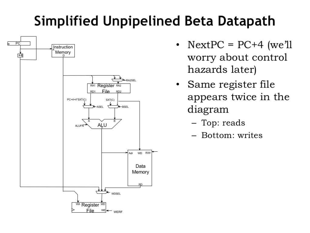
Let’s start by redrawing and simplifying the Beta data path so that it will be easier to reason about when we add pipelining.
The first simplification is to focus on sequential execution and so leave out the branch addressing and PC MUX logic. Our simplified Beta always executes the next instruction from PC+4. We’ll add back the branch and jump logic when we discuss control hazards.
The second simplification is to have the register file appear twice in the diagram so that we can tease apart the read and write operations that occur at different stages of instruction execution. The top Register File shows the combinational read ports, used when reading the register operands in the RF stage. The bottom Register File shows the clocked write port, used to write the result into the destination register at the end of the WB stage. Physically, there’s only one set of 32 registers, we’ve just drawn the read and write circuity as separate components in the diagram.
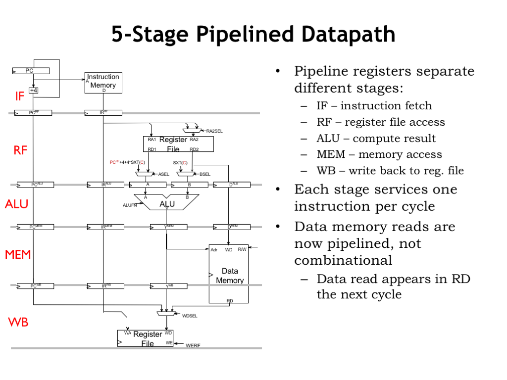
If we add pipeline registers to the simplified diagram, we see that execution proceeds through the five stages from top to bottom. If we consider execution of instruction sequences with no data hazards, information is flowing down the pipeline and the pipeline will correctly overlap the execution of all the instructions in the pipeline.
The diagram shows the components needed to implement each of the five stages. The IF stage contains the program counter and the main memory interface for fetching instructions. The RF stage has the register file and operand multiplexers. The ALU stage uses the operands and computes the result. The MEM stage handles the memory access for load and store operations. And the WB stage writes the result into the destination register.
In each clock cycle, each stage does its part in the execution of a particular instruction. In a given clock cycle, there are 5 instructions in the pipeline.
Note that data accesses to main memory span almost two clock cycles. Data accesses are initiated at the beginning of the MEM stage and returning data is only needed just before the end of the WB stage. The memory is itself pipelined and can simultaneously finish the access from an earlier instruction while starting an access for the next instruction.
This simplified diagram isn’t showing how the control logic is split across the pipeline stages. How does that work?
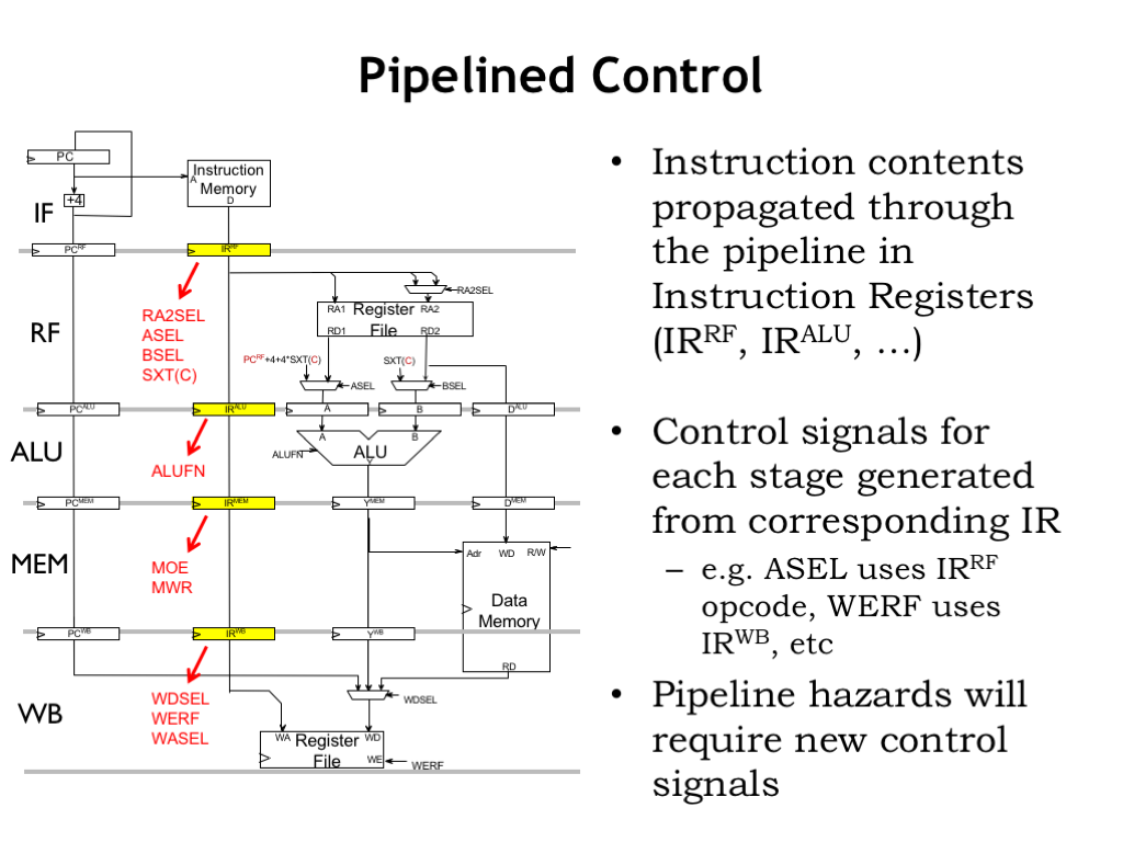
Note that we’ve included instruction registers as part of each pipeline stage, so that each stage can compute the control signals it needs from its instruction register. The encoded instruction is simply passed from one stage to the next as the instruction flows through the pipeline.
Each stage computes its control signals from the opcode field of its instruction register. The RF stage needs the RA, RB, and literal fields from its instruction register. And the WB stage needs the RC field from its instruction register. The required logic is very similar to the unpipelined implementation, it’s just been split up and moved to the appropriate pipeline stage.
We’ll see that we will have to add some additional control logic to deal correctly with pipeline hazards.
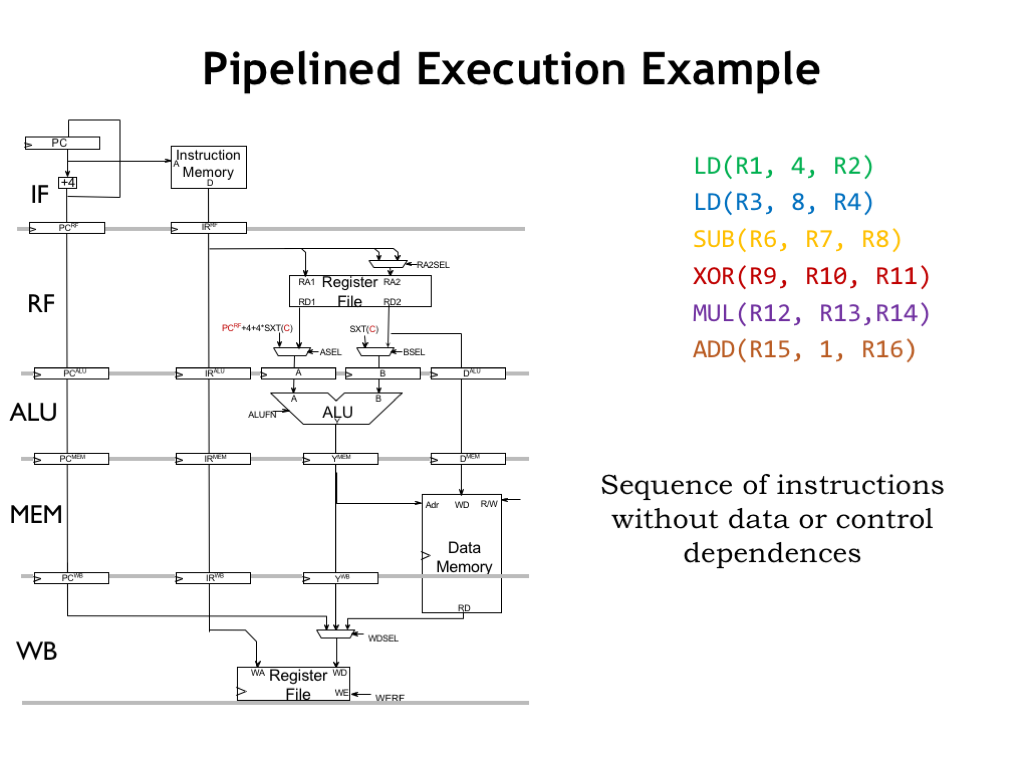
Our simplified diagram isn’t so simple anymore! To see how the pipeline works, let’s follow along as it executes this sequence of six instructions. Note that the instructions are reading and writing from different registers, so there are no potential data hazards. And there are no branches and jumps, so there are no potential control hazards. Since there are no potential hazards, the instruction executions can be overlapped and their overlapped execution in the pipeline will work correctly.
Okay, here we go!
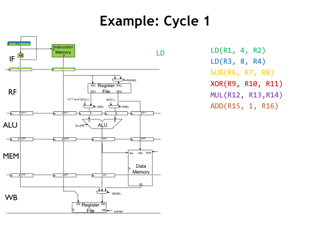
During cycle 1, the IF stage sends the value from the program counter to main memory to fetch the first instruction (the green LD instruction), which will be stored in the RF-stage instruction register at the end of the cycle. Meanwhile, it’s also computing PC+4, which will be the next value of the program counter. We’ve colored the next value blue to indicate that it’s the address of the blue instruction in the sequence.
We’ll add the appropriately colored label on the right of each pipeline stage to indicate which instruction the stage is processing.
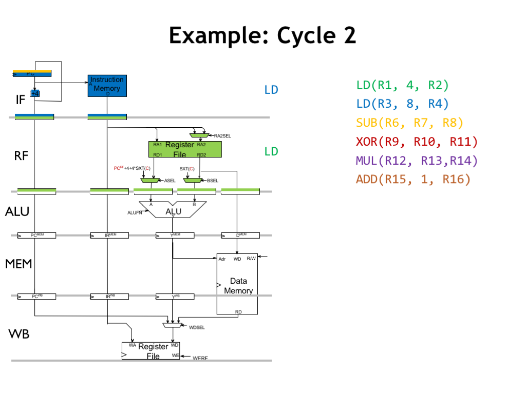
At the start of cycle 2, we see that values in the PC and instruction registers for the RF stage now correspond to the green instruction. During the cycle the register file will be reading the register operands, in this case R1, which is needed for the green instruction. Since the green instruction is a LD, ASEL is 0 and BSEL is 1, selecting the appropriate values to be written into the A and B operand registers at the end of the cycle.
Concurrently, the IF stage is fetching the blue instruction from main memory and computing an updated PC value for the next cycle.
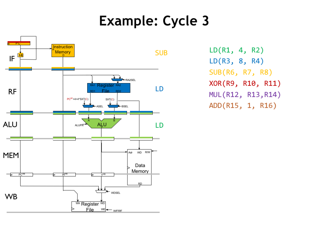
In cycle 3, the green instruction is now in the ALU stage, where the ALU is adding the values in its operand registers (in this case the value of R1 and the constant 4) and the result will be stored in Y_MEM register at the end of the cycle.
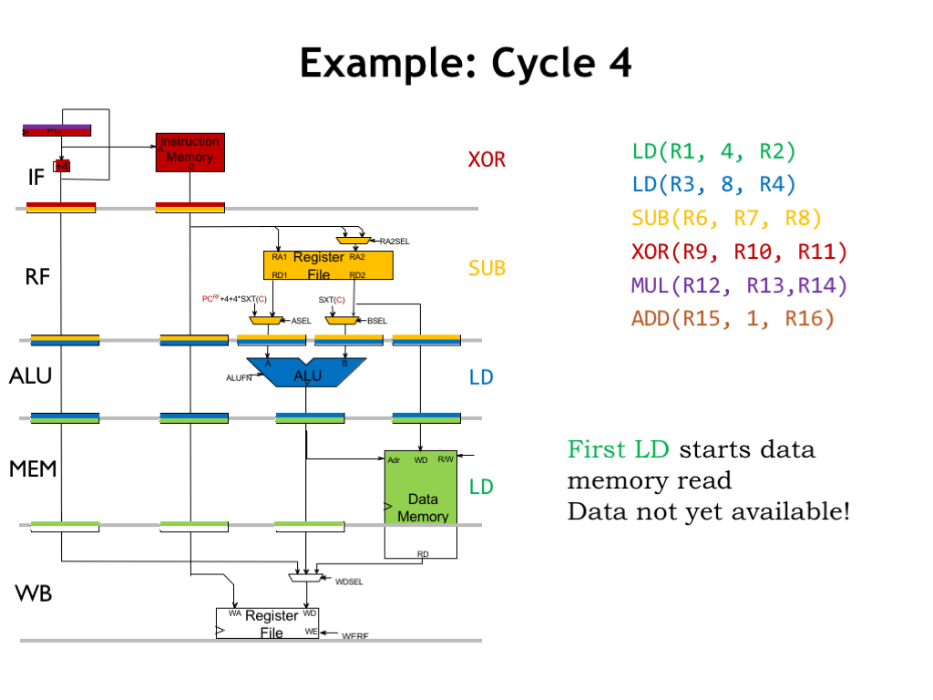
In cycle 4, we’re overlapping the execution of four instructions. The MEM stage initiates a memory read for the green LD instruction. Note that the read data will first become available in the WB stage - it’s not available to CPU in the current clock cycle.
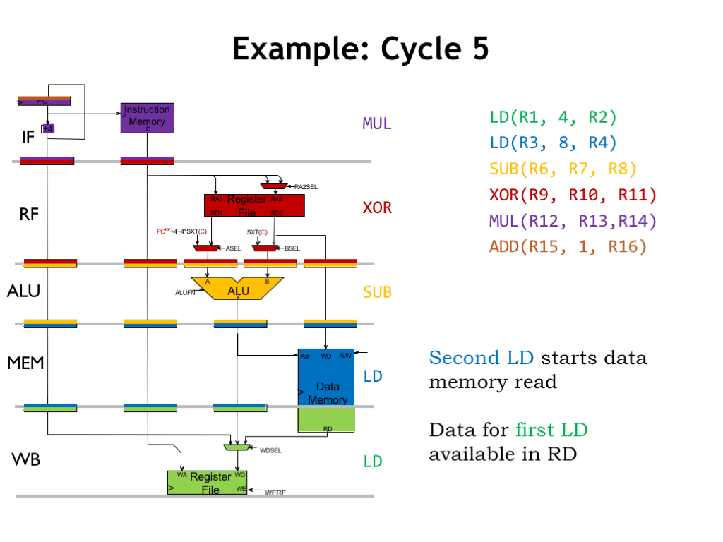
In cycle 5, the results of the main memory read initiated in cycle 4 are available for writing to the register file in the WB stage. So execution of the green LD instruction will be complete when the memory data is written to R2 at the end of cycle 5.
Meanwhile, the MEM stage is initiating a memory read for the blue LD instruction.
The pipeline continues to complete successive instructions in successive clock cycles. The latency for a particular instruction is 5 clock cycles. The throughput of the pipelined CPU is 1 instruction/cycle. This is the same as the unpipelined implementation, except that the clock period is shorter because each pipeline stage has fewer components.
Note that the effects of the green LD, i.e., filling R2 with a new value, don’t happen until the rising edge of the clock at the end of cycle 5. In other words, the results of the green LD aren’t available to other instructions until cycle 6. If there were instructions in the pipeline that read R2 before cycle 6, they would have gotten an old value! This is an example of a data hazard. Not a problem for us, since our instruction sequence didn’t trigger this data hazard.
Tackling data hazards is our next task.
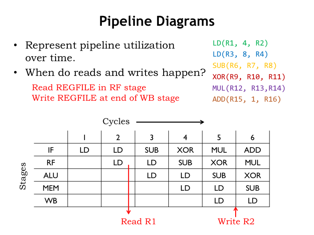
The data path diagram isn’t all that useful in diagramming the pipelined execution of an instruction sequence since we need a new copy of the diagram for each clock cycle. A more compact and easier-to-read diagram of pipelined execution is provided by the pipeline diagrams we met back in Part 1 of the course.
There’s one row in the diagram for each pipeline stage and one column for each cycle of execution. Entries in the table show which instruction is in each pipeline stage at each cycle. In normal operation, a particular instruction moves diagonally through the diagram as it proceeds through the five pipeline stages.
To understand data hazards, let’s first remind ourselves of when the register file is read and written for a particular instruction. Register reads happen when the instruction is in the RF stage, i.e., when we’re reading the instruction’s register operands. Register writes happen at the end of the cycle when the instruction is in the WB stage. For example, for the first LD instruction, we read R1 during cycle 2 and write R2 at the end of cycle 5. Or consider the register file operations in cycle 6: we’re reading R12 and R13 for the MUL instruction in the RF stage, and writing R4 at the end of the cycle for the LD instruction in the WB stage.
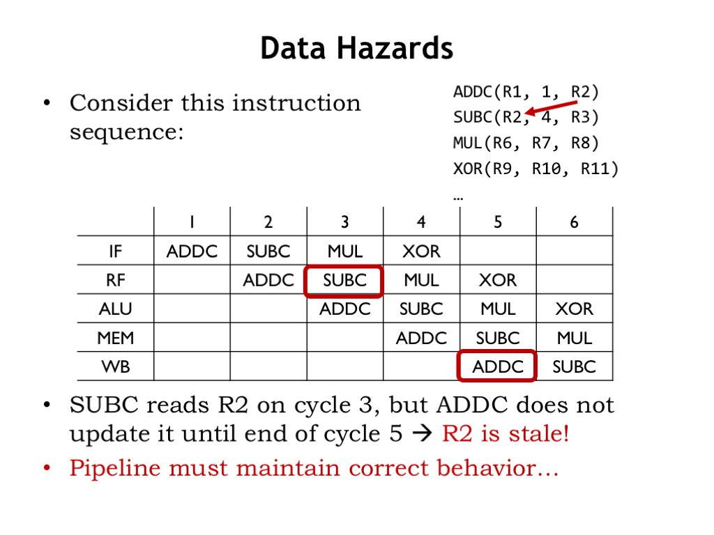
Okay, now let’s see what happens when there are data hazards. In this instruction sequence, the ADDC instruction writes its result in R2, which is immediately read by the following SUBC instruction. Correct execution of the SUBC instruction clearly depends on the results of the ADDC instruction. This what we’d call a read-after-write dependency.
This pipeline diagram shows the cycle-by-cycle execution where we’ve circled the cycles during which ADDC writes R2 and SUBC reads R2.
Oops! ADDC doesn’t write R2 until the end of cycle 5, but SUBC is trying to read the R2 value in cycle 3. The value in R2 in the register file in cycle 3 doesn’t yet reflect the execution of the ADDC instruction. So as things stand the pipeline would *not* correctly execute this instruction sequence. This instruction sequence has triggered a data hazard.
We want the pipelined CPU to generate the same program results as the unpipelined CPU, so we’ll need to figure out a fix.
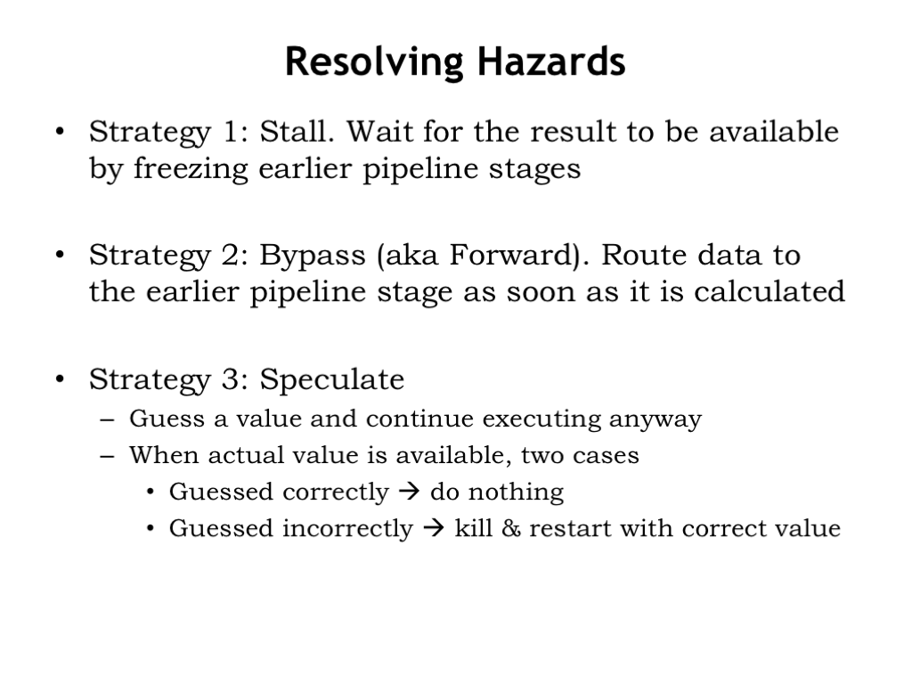
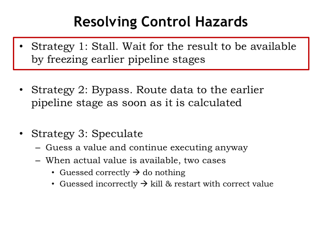
There are three general strategies we can pursue to fix pipeline hazards. Any of the techniques will work, but as we’ll see they have different tradeoffs for instruction throughput and circuit complexity.
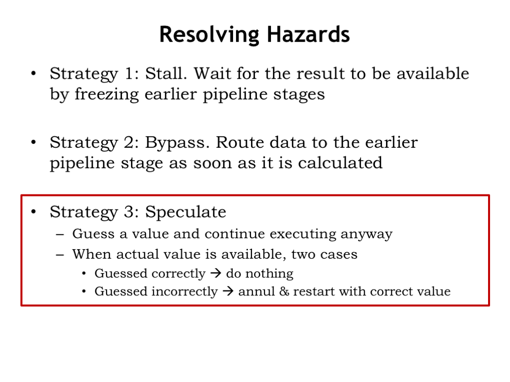
The first strategy is to stall instructions in the RF stage until the result they need has been written to the register file. “Stall” means that we don’t reload the instruction register at the end of the cycle, so we’ll try to execute the same instruction in the next cycle. If we stall one pipeline stage, all earlier stages must also be stalled since they are blocked by the stalled instruction. If an instruction is stalled in the RF stage, the IF stage is also stalled. Stalling will always work, but has a negative impact on instruction throughput. Stall for too many cycles and you’ll lose the performance advantages of pipelined execution!
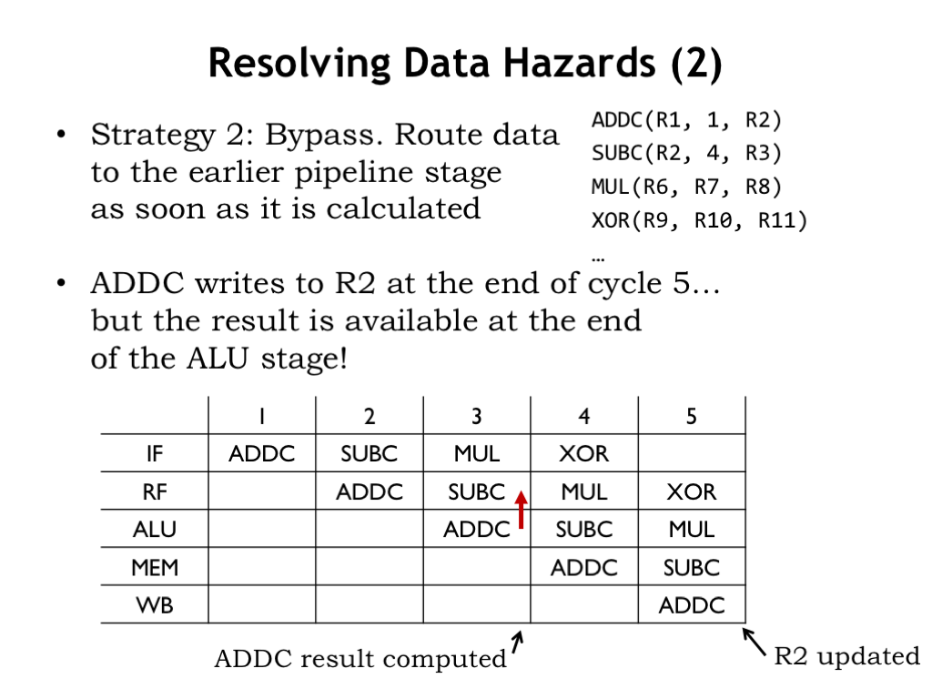
The second strategy is to route the needed value to earlier pipeline stages as soon as its computed. This called bypassing or forwarding. As it turns out, the value we need often exists somewhere in the pipelined data path, it just hasn’t been written yet to the register file. If the value exists and can be forwarded to where it’s needed, we won’t need to stall. We’ll be able to use this strategy to avoid stalling on most types of data hazards.
The third strategy is called speculation. We’ll make an intelligent guess for the needed value and continue execution. Once the actual value is determined, if we guessed correctly, we’re all set. If we guessed incorrectly, we have to back up execution and restart with the correct value. Obviously speculation only makes sense if it’s possible to make accurate guesses. We’ll be able to use this strategy to avoid stalling on control hazards.
Let’s see how the first two strategies work when dealing with our data hazard.
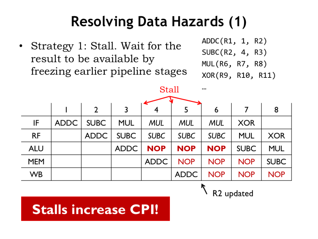
Applying the stall strategy to our data hazard, we need to stall the SUBC instruction in the RF stage until the ADDC instruction writes its result in R2. So in the pipeline diagram, SUBC is stalled three times in the RF stage until it can finally access the R2 value from the register file in cycle 6.
Whenever the RF stage is stalled, the IF stage is also stalled. You can see that in the diagram too. But when RF is stalled, what should the ALU stage do in the next cycle? The RF stage hasn’t finished its job and so can’t pass along its instruction! The solution is for the RF stage to make-up an innocuous instruction for the ALU stage, what’s called a NOP instruction, short for “no operation”. A NOP instruction has no effect on the CPU state, i.e., it doesn’t change the contents of the register file or main memory. For example any OP-class or OPC-class instruction that has R31 as its destination register is a NOP.
The NOPs introduced into the pipeline by the stalled RF stage are shown in red. Since the SUBC is stalled in the RF stage for three cycles, three NOPs are introduced into the pipeline. We sometimes refer to these NOPs as “bubbles” in the pipeline.
How does the pipeline know when to stall? It can compare the register numbers in the RA and RB fields of the instruction in the RF stage with the register numbers in the RC field of instructions in the ALU, MEM, and WB stage. If there’s a match, there’s a data hazard and the RF stage should be stalled. The stall will continue until there’s no hazard detected. There are a few details to take care of: some instructions don’t read both registers, the ST instruction doesn’t use its RC field, and we don’t want R31 to match since it’s always okay to read R31 from the register file.
Stalling will ensure correct pipelined execution, but it does increase the effective CPI. This will lead to longer execution times if the increase in CPI is larger than the decrease in cycle time afforded by pipelining.
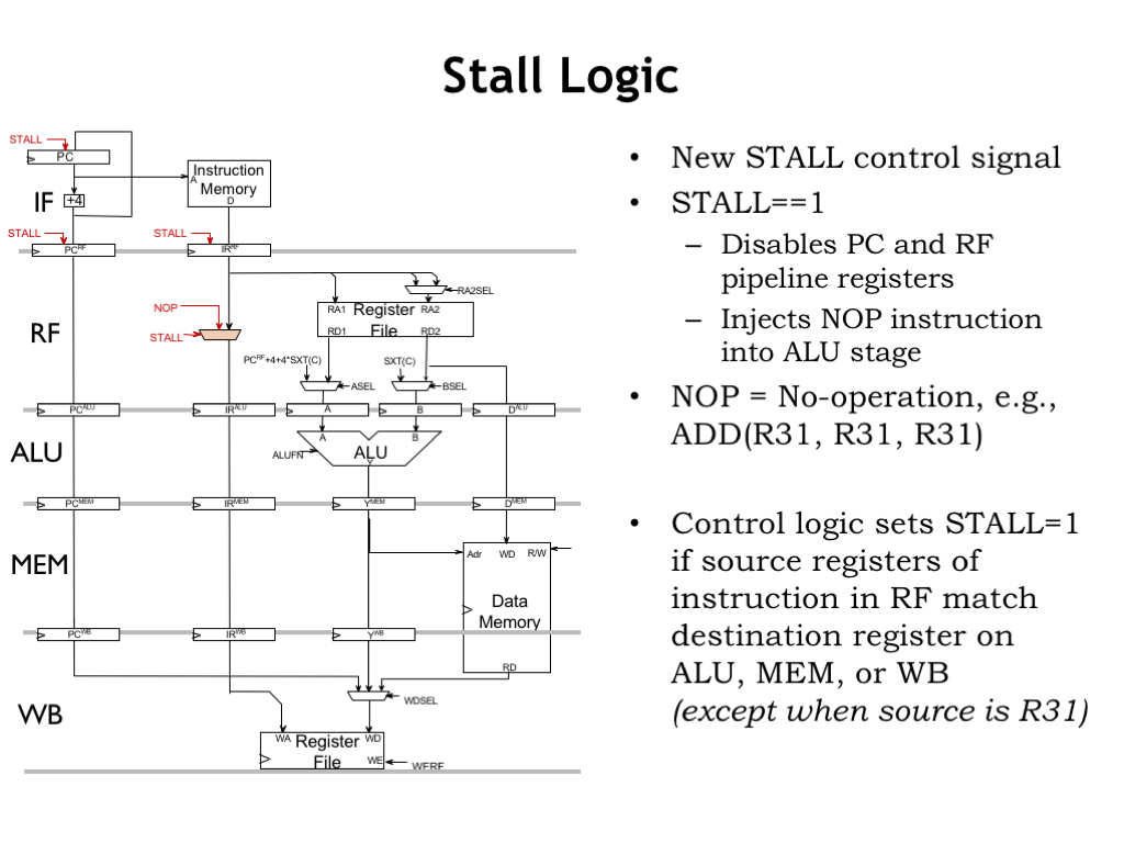
To implement stalling, we only need to make two simple changes to our pipelined data path. We generate a new control signal, STALL, which, when asserted, disables the loading of the three pipeline registers at the input of the IF and RF stages, which means they’ll have the same value next cycle as they do this cycle. We also introduce a mux to choose the instruction to be sent along to the ALU stage. If STALL is 1, we choose a NOP instruction, e.g., an ADD with R31 as its destination. If STALL is 0, the RF stage is not stalled, so we pass its current instruction to the ALU.
And here we see how to compute STALL as described in the previous slide.
The additional logic needed to implement stalling is pretty modest, so the real design tradeoff is about increased CPI due to stalling vs. decreased cycle time due to pipelining.
So we have a solution, although it carries some potential performance costs.
Now let’s consider our second strategy: bypassing, which is applicable if the data we need in the RF stage is somewhere in the pipelined data path.
In our example, even though ADDC doesn’t write R2 until the end of cycle 5, the value that will be written is computed during cycle 3 when the ADDC is in the ALU stage. In cycle 3, the output of the ALU is the value needed by the SUBC that’s in the RF stage in the same cycle.
So, if we detect that the RA field of the instruction in the RF stage is the same as the RC field of the instruction in the ALU stage, we can use the output of the ALU in place of the (stale) RA value being read from the register file. No stalling necessary!
In our example, in cycle 3 we want to route the output of the ALU to the RF stage to be used as the value for R2. We show this with a red “bypass arrow” showing data being routed from the ALU stage to the RF stage.
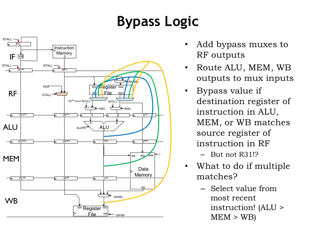
To implement bypassing, we’ll add a many-input multiplexer to the read ports of the register file so we can select the appropriate value from other pipeline stages. Here we show the combinational bypass paths from the ALU, MEM, and WB stages. For the bypassing example of previous slides, we use the blue bypass path during cycle 3 to get the correct value for R2.
The bypass MUXes are controlled by logic that’s matching the number of the source register to the number of the destination registers in the ALU, MEM, and WB stages, with the usual complications of dealing with R31.
What if there are multiple matches, i.e., if the RF stage is trying to read a register that’s the destination for, say, the instructions in both the ALU and MEM stages? No problem! We want to select the result from the most recent instruction, so we’d choose the ALU match if there is one, then the MEM match, then the WB match, then, finally, the output of the register file.

Here’s a diagram showing all the bypass paths we’ll need. Note that branches and jumps write their PC+4 value into the register file, so we’ll need to bypass from the PC+4 values in the various stages as well as the ALU values.
Note that the bypassing is happening at the end of the cycle, e.g., after the ALU has computed its answer. To accommodate the extra t_PD of the bypass MUX, we’ll have to extend the clock period by a small amount. So once again there’s a design tradeoff - the increased CPI of stalling vs the slightly increased cycle time of bypassing. And, of course, in the case of bypassing there’s the extra area needed for the necessary wiring and MUXes.
We can cut back on the costs by reducing the amount of bypassing, say, to only bypassing ALU results from the ALU stage and use stalling to deal with all the other data hazards.
If we implement full bypassing, do we still need the STALL logic?
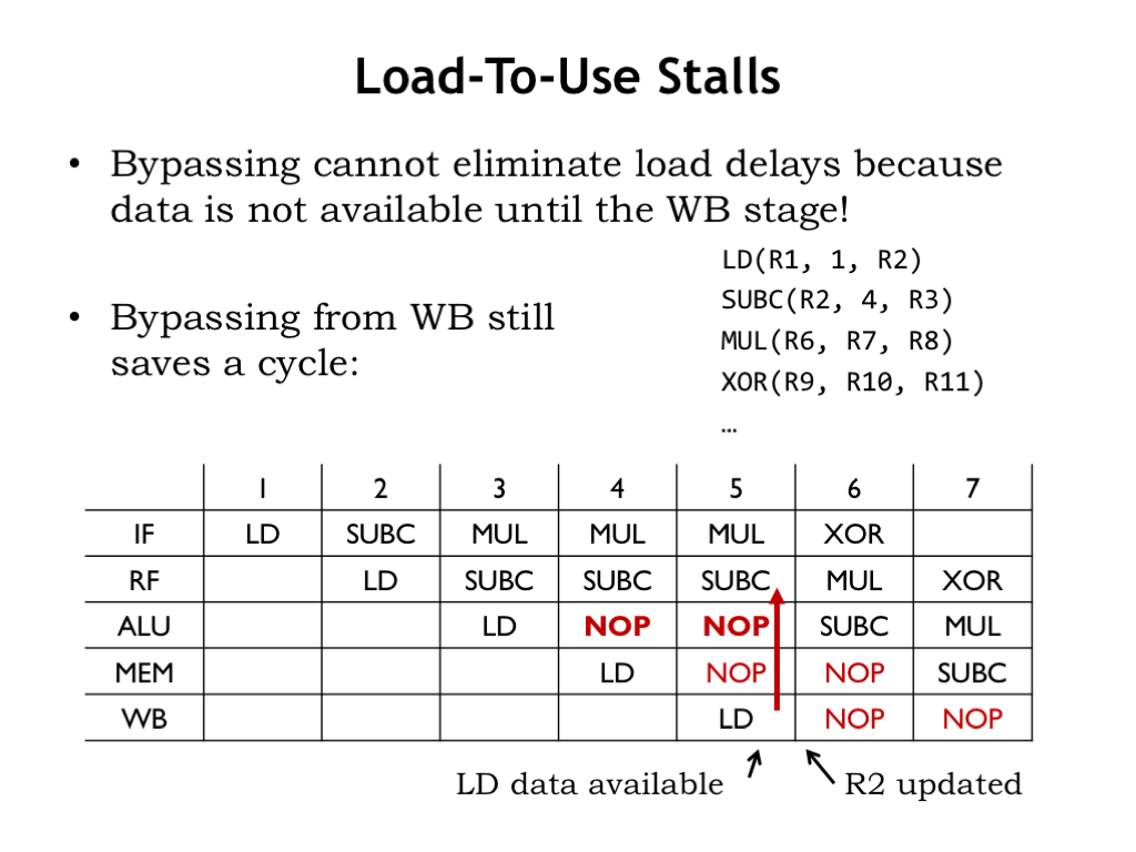
As it turns out, we do! There’s one data hazard that bypassing doesn’t completely address. Consider trying to immediately the use the result of a LD instruction. In the example shown here, the SUBC is trying to use the value the immediately preceding LD is writing to R2. This is called a load-to-use hazard.
Recalling that LD data isn’t available in the data path until the cycle when LD reaches the WB stage, even with full bypassing we’ll need to stall SUBC in the RF stage until cycle 5, introducing two NOPs into the pipeline. Without bypassing from the WB stage, we need to stall until cycle 6.

In summary, we have two strategies for dealing with data hazards.
We can stall the IF and RF stages until the register values needed by the instruction in the RF stage are available in the register file. The required hardware is simple, but the NOPs introduced into the pipeline waste CPU cycles and result in an higher effective CPI.
Or we can use bypass paths to route the required values to the RF stage assuming they exist somewhere in the pipelined data path. This approach requires more hardware than stalling, but doesn’t reduce the effective CPI. Even if we implement bypassing, we’ll still need stalls to deal with load-to-use hazards.
Can we keep adding pipeline stages in the hopes of further reducing the clock period? More pipeline stages mean more instructions in the pipeline at the same time, which in turn increases the chance of a data hazard and the necessity of stalling, thus increasing CPI.
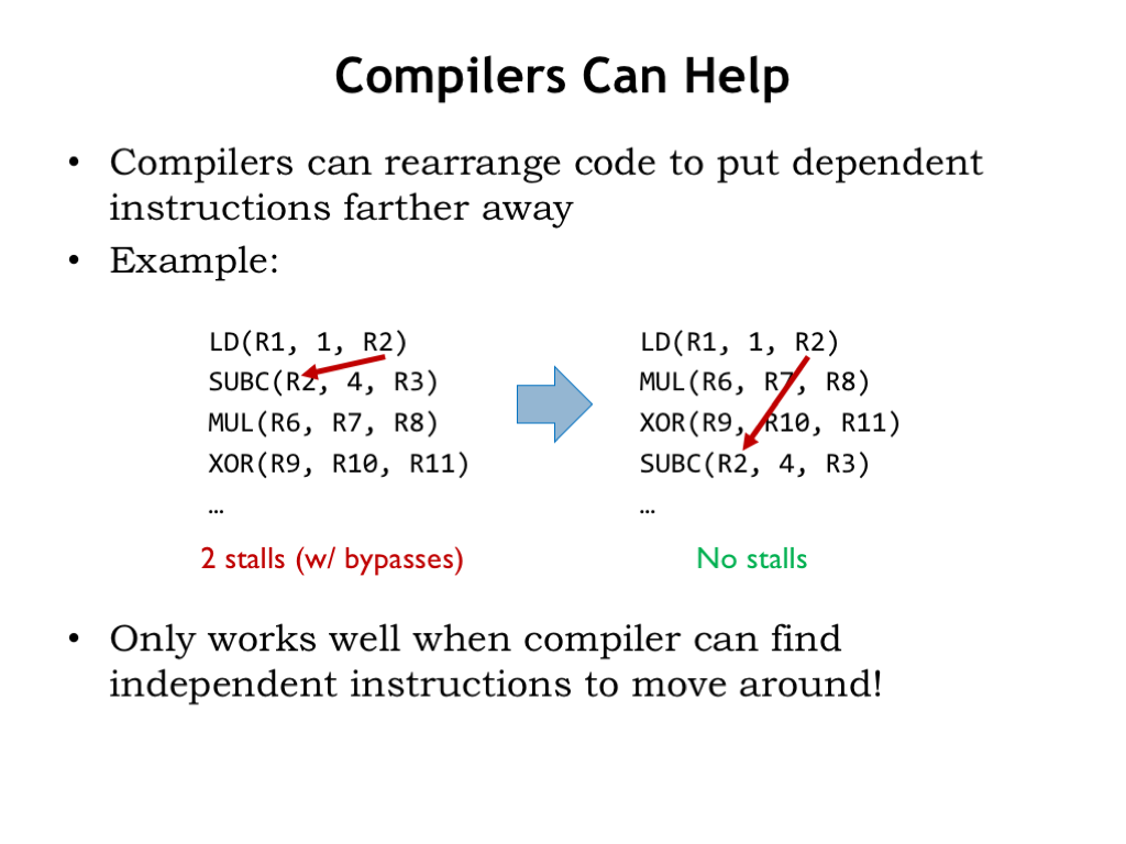
Compilers can help reduce dependencies by reorganizing the assembly language code they produce. Here’s the load-to-use hazard example we saw earlier. Even with full bypassing, we’d need to stall for 2 cycles.
But if the compiler (or assembly language programmer!) notices that the MUL and XOR instructions are independent of the SUBC instruction and hence can be moved before the SUBC, the dependency is now such that the LD is naturally in the WB stage when the ST is in the RF stage, so no stalls are needed.
This optimization only works when the compiler can find independent instructions to move around. Unfortunately there are plenty of programs where such instructions are hard to find.
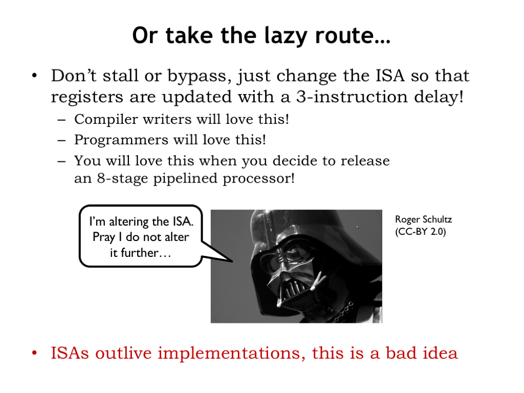
Then there’s one final approach we could take - change the ISA so that data hazards are part of the ISA, i.e., just explain that writes to the destination register happen with a 3-instruction delay! If NOPs are needed, make the programmer add them to the program. Simplify the hardware at the “small” cost of making the compilers work harder.
You can imagine exactly how much the compiler writers will like this suggestion. Not to mention assembly language programmers! And you can change the ISA again when you add more pipeline stages!
This is how a compiler writer views CPU architects who unilaterally change the ISA to save a few logic gates :)
The bottom line is that successful ISAs have very long lifetimes and so shouldn’t include tradeoffs driven by short-term implementation considerations. Best not to go there.
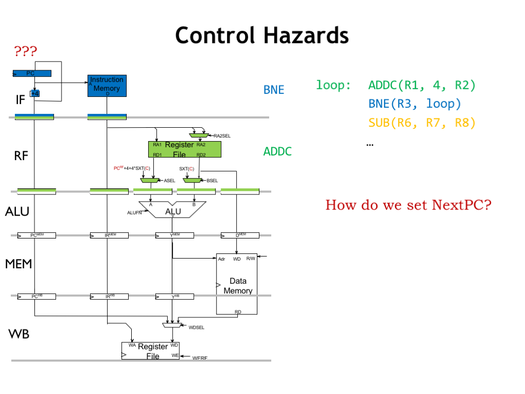
Now let’s turn our attention to control hazards, illustrated by the code fragment shown here. Which instruction should be executed after the BNE? If the value in R3 is non-zero, ADDC should be executed. If the value in R3 is zero, the next instruction should be SUB. If the current instruction is an explicit transfer of control (i.e., JMPs or branches), the choice of the next instruction depends on the execution of the current instruction.
What are the implications of this dependency on our execution pipeline?
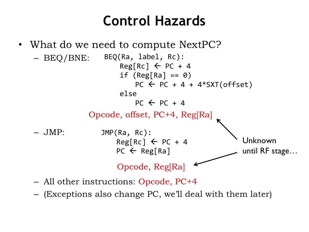
How does the unpipelined implementation determine the next instruction?
For branches (BEQ or BNE), the value to be loaded into the program counter depends on (1) the opcode, i.e., whether the instruction is a BEQ or a BNE, (2) the current value of the program counter since that’s used in the offset calculation, and (3) the value stored in the register specified by the RA field of the instruction since that’s the value tested by the branch.
For JMP instructions, the next value of the program counter depends once again on the opcode field and the value of the RA register.
For all other instructions, the next PC value depends only on the opcode of the instruction and the value PC+4.
Exceptions also change the program counter. We’ll deal with them later in the lecture.
The control hazard is triggered by JMP and branches since their execution depends on the value in the RA register, i.e., they need to read from the register file, which happens in the RF pipeline stage. Our bypass mechanisms ensure that we’ll use the correct value for the RA register even if it’s not yet been written into the register file. What we’re concerned about here is that the address of the instruction following the JMP or branch will be loaded into program counter at the end of the cycle when the JMP or branch is in the RF stage. But what should the IF stage be doing while all this is going on in RF stage?
The answer is that in the case of JMPs and taken branches, we don’t know what the IF stage should be doing until those instructions are able to access the value of the RA register in the RF stage.
One solution is to stall the IF stage until the RF stage can compute the necessary result. This was the first of our general strategies for dealing with hazards. How would this work?
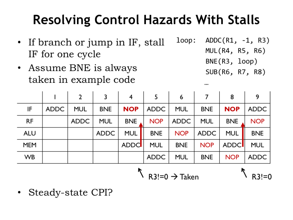
If the opcode in the RF stage is JMP, BEQ, or BNE, stall the IF stage for one cycle. In the example code shown here, assume that the value in R3 is non-zero when the BNE is executed, i.e., that the instruction following BNE should be the ADDC at the top of the loop.
The pipeline diagram shows the effect we’re trying to achieve: a NOP is inserted into the pipeline in cycles 4 and 8. Then execution resumes in the next cycle after the RF stage determines what instruction comes next. Note, by the way, that we’re relying on our bypass logic to deliver the correct value for R3 from the MEM stage since the ADDC instruction that wrote into R3 is still in the pipeline, i.e., we have a data hazard to deal with too!
Looking at, say, the WB stage in the pipeline diagram, we see it takes 4 cycles to execute one iteration of our 3-instruction loop. So the effective CPI is 4/3, an increase of 33%. Using stall to deal with control hazards has had an impact on the instruction throughput of our execution pipeline.
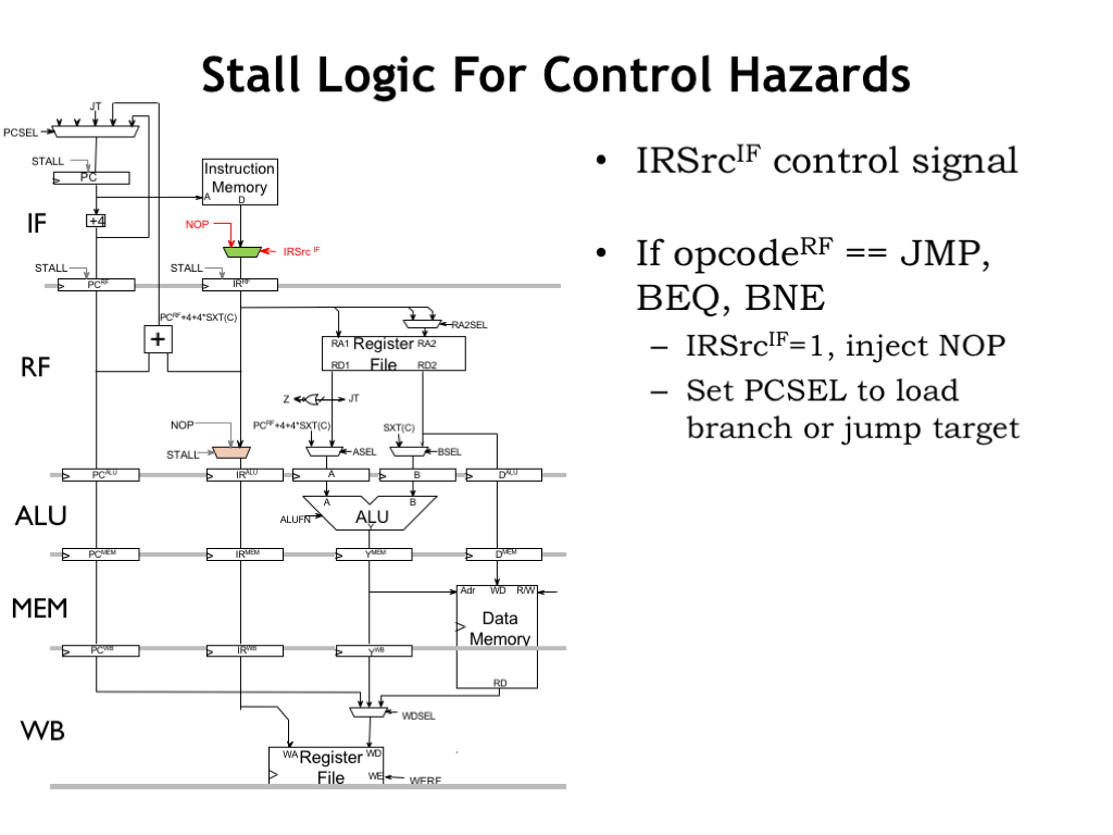
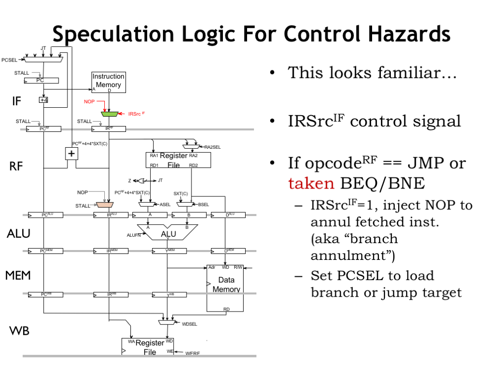
We’ve already seen the logic needed to introduce NOPs into the pipeline. In this case, we add a mux to the instruction path in the IF stage, controlled by the IRSrc_IF select signal. We use the superscript on the control signals to indicate which pipeline stage holds the logic they control.
If the opcode in the RF stage is JMP, BEQ, or BNE we set IRSrc_IF to 1, which causes a NOP to replace the instruction that was being read from main memory. And, of course, we’ll be setting the PCSEL control signals to select the correct next PC value, so the IF stage will fetch the desired follow-on instruction in the next cycle.
If we replace an instruction with NOP, we say we “annulled” the instruction.
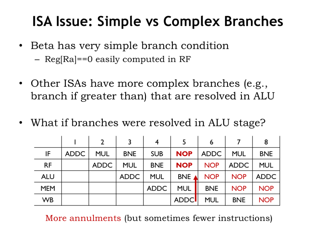
The branch instructions in the Beta ISA make their branch decision in the RF stage since they only need the value in register RA.
But suppose the ISA had a branch where the branch decision was made in ALU stage.
When the branch decision is made in the ALU stage, we need to introduce two NOPs into the pipeline, replacing the now unwanted instructions in the RF and IF stages. This would increase the effective CPI even further. But the tradeoff is that the more complex branches may reduce the number of instructions in the program.
If we annul instructions in all the earlier pipeline stages, this is called “flushing the pipeline”. Since flushing the pipeline has a big impact on the effective CPI, we do it when it’s the only way to ensure the correct behavior of the execution pipeline.
We can be smarter about when we choose to flush the pipeline when executing branches. If the branch is not taken, it turns out that the pipeline has been doing the right thing by fetching the instruction following the branch. Starting execution of an instruction even when we’re unsure whether we really want it executed is called “speculation”.
Speculative execution is okay if we’re able to annul the instruction before it has an effect on the CPU state, e.g., by writing into the register file or main memory. Since these state changes (called “side effects”) happen in the later pipeline stages, an instruction can progress through the IF, RF, and ALU stages before we have to make a final decision about whether it should be annulled.
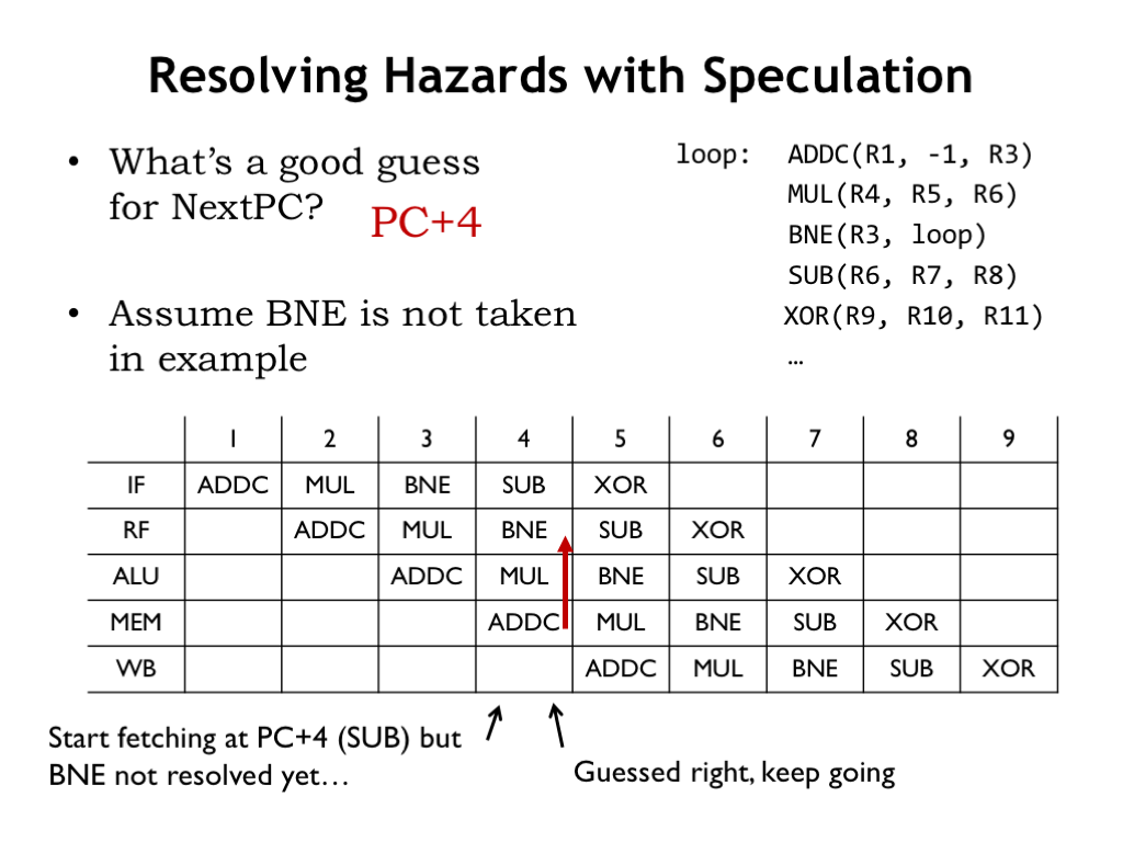
How does speculation help with control hazards? Guessing that the next value of the program counter is PC+4 is correct for all but JMPs and taken branches.
Here’s our example again, but this time let’s assume that the BNE is not taken, i.e., that the value in R3 is zero. The SUB instruction enters the pipeline at the start of cycle 4. At the end of cycle 4, we know whether or not to annul the SUB. If the branch is not taken, we want to execute the SUB instruction, so we just let it continue down the pipeline.
In other words, instead of always annulling the instruction following branch, we only annul it if the branch was taken. If the branch is not taken, the pipeline has speculated correctly and no instructions need to be annulled.

However if the BNE is taken, the SUB is annulled at the end of cycle 4 and a NOP is executed in cycle 5. So we only introduce a bubble in the pipeline when there’s a taken branch. Fewer bubbles will decrease the impact of annulment on the effective CPI.
We’ll be using the same data path circuitry as before, we’ll just be a bit more clever about when the value of the IRSrc_IF control signal is set to 1. Instead of setting it to 1 for all branches, we only set it to 1 when the branch is taken.
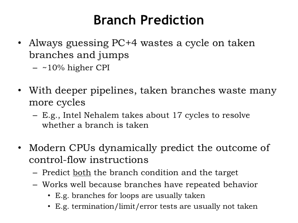
Our naive strategy of always speculating that the next instruction comes from PC+4 is wrong for JMPs and taken branches. Looking at simulated execution traces, we’ll see that this error in speculation leads to about 10% higher effective CPI. Can we do better?
This is an important question for CPUs with deep pipelines. For example, Intel’s Nehalem processor from 2009 resolves the more complex x86 branch instructions quite late in the pipeline. Since Nehalem is capable of executing multiple instructions each cycle, flushing the pipeline in Nehalem actually annuls the execution of many instructions, resulting in a considerable hit on the CPI.
Like many modern processor implementations, Nehalem has a much more sophisticated speculation mechanism. Rather than always guessing the next instruction is at PC+4, it only does that for non-branch instructions. For branches, it predicts the behavior of each individual branch based on what the branch did last time it was executed and some knowledge of how the branch is being used. For example, backward branches at the end of loops, which are taken for all but the final iteration of the loop, can be identified by their negative branch offset values. Nehalem can even determine if there’s correlation between branch instructions, using the results of an another, earlier branch to speculate on the branch decision of the current branch. With these sophisticated strategies, Nehalem’s speculation is correct 95% to 99% of the time, greatly reducing the impact of branches on the effective CPI.
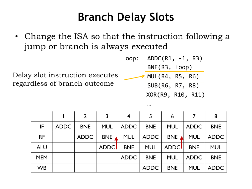
There’s also the lazy option of changing the ISA to deal with control hazards. For example, we could change the ISA to specify that the instruction following a jump or branch is always executed. In other words the transfer of control happens *after* the next instruction. This change ensures that the guess of PC+4 as the address of the next instruction is always correct!
In the example shown here, assuming we changed the ISA, we can reorganize the execution order of the loop to place the MUL instruction after the BNE instruction, in the so-called “branch delay slot”. Since the instruction in the branch delay slot is always executed, the MUL instruction will be executed during each iteration of the loop.
The resulting execution is shown in this pipeline diagram. Assuming we can find an appropriate instruction to place in the branch delay slot, the branch will have zero impact on the effective CPI.
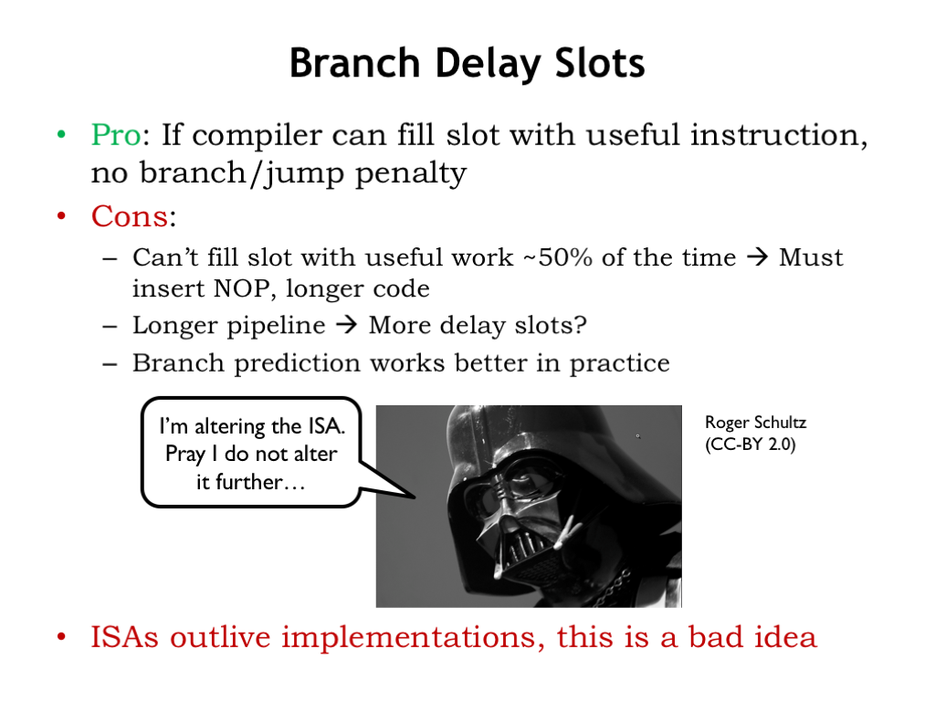
Are branch delay slots a good idea? Seems like they reduce the negative impact that branches might have on instruction throughput.
The downside is that only half the time can we find instructions to move to the branch delay slot. The other half of the time we have to fill it with an explicit NOP instruction, increasing the size of the code. And if we make the branch decision later in the pipeline, there are more branch delay slots, which would be even harder to fill. In practice, it turns out that branch prediction works better than delay slots in reducing the impact of branches.
So, once again we see that it’s problematic to alter the ISA to improve the throughput of pipelined execution. ISAs outlive implementations, so it’s best not to change the execution semantics to deal with performance issues created by a particular implementation.

Now let’s figure out how exceptions impact pipelined execution. When an exception occurs because of an illegal instruction or an external interrupt, we need to store the current PC+4 value in the XP register and load the program counter with the address of the appropriate exception handler.
Exceptions cause control flow hazards since they are effectively implicit branches.
In an unpipelined implementation, exceptions affect the execution of the current instruction. We want to achieve exactly the same effect in our pipelined implementation. So first we have to identify which one of the instructions in our pipeline is affected, then ensure that instructions that came earlier in the code complete correctly and that we annul the affected instruction and any following instructions that are in the pipeline.
Since there are multiple instructions in the pipeline, we have a bit of sorting out to do.
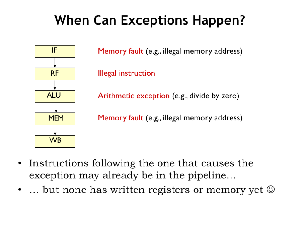
When, during pipelined execution, do we determine that an instruction will cause an exception? An obvious example is detecting an illegal opcode when we decode the instruction in the RF stage. But we can also generate exceptions in other pipeline stages. For example, the ALU stage can generate an exception if the second operand of a DIV instruction is 0. Or the MEM stage may detect that the instruction is attempting to access memory with an illegal address. Similarly the IF stage can generate a memory exception when fetching the next instruction.
In each case, instructions that follow the one that caused the exception may already be in the pipeline and will need to be annulled. The good news is that since register values are only updated in the WB stage, annulling an instruction only requires replacing it with a NOP. We won’t have to restore any changed values in the register file or main memory.
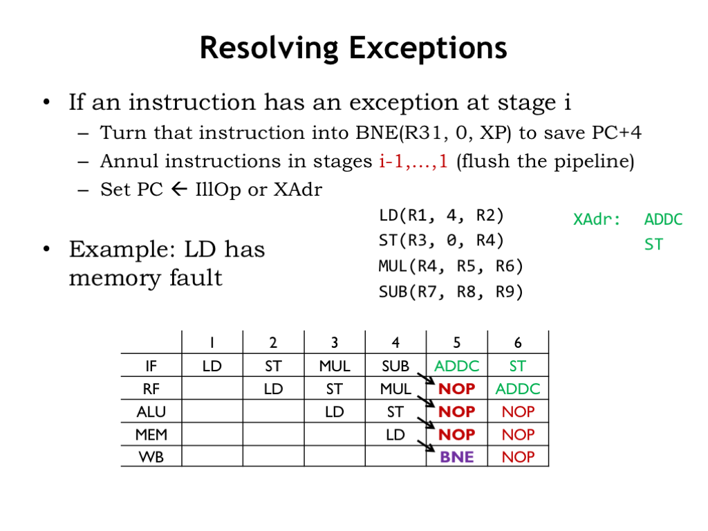
Here’s our plan. If an instruction causes an exception in stage i, replace that instruction with this BNE instruction, whose only side effect is writing the PC+4 value into the XP register. Then flush the pipeline by annulling instructions in earlier pipeline stages. And, finally, load the program counter with the address of the exception handler.
In this example, assume that LD will generate a memory exception in the MEM stage, which occurs in cycle 4. The arrows show how the instructions in the pipeline are rewritten for cycle 5, at which point the IF stage is working on fetching the first instruction in the exception handler.
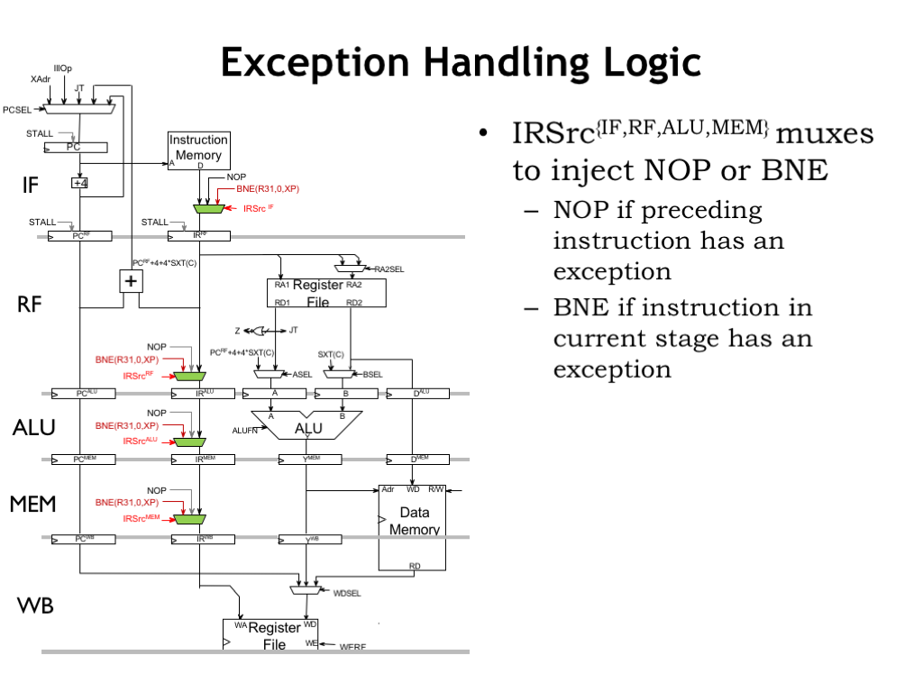
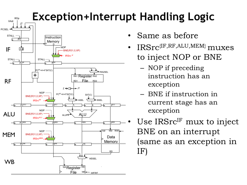
Here are the changes required to the execution pipeline. We modify the muxes in the instruction path so that they can replace an actual instruction with either NOP if the instruction is to be annulled, or BNE if the instruction caused the exception.
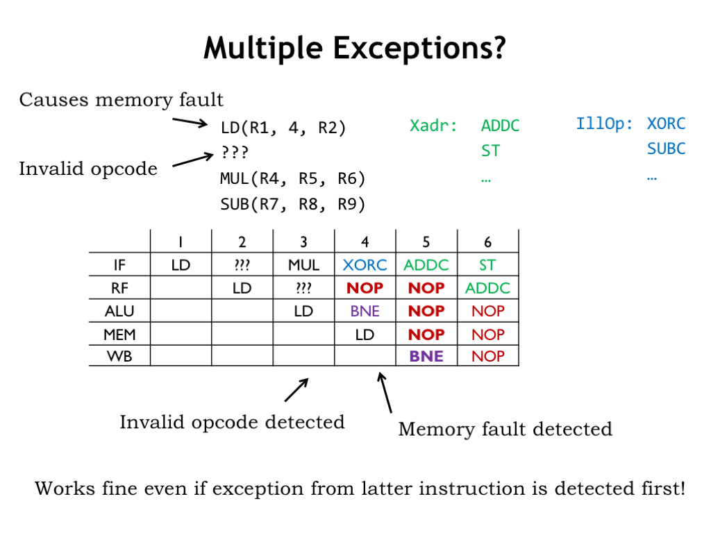
Since the pipeline is executing multiple instructions at the same time, we have to worry about what happens if multiple exceptions are detected during execution. In this example assume that LD will cause a memory exception in the MEM stage and note that it is followed by an instruction with an illegal opcode.
Looking at the pipeline diagram, the invalid opcode is detected in the RF stage during cycle 3, causing the illegal instruction exception process to begin in cycle 4. But during that cycle, the MEM stage detects the illegal memory access from the LD instruction and so causes the memory exception process to begin in cycle 5. Note that the exception caused by the earlier instruction (LD) overrides the exception caused by the later illegal opcode even though the illegal opcode exception was detected first. That’s the correct behavior since once the execution of LD is abandoned, the pipeline should behave as if none of the instructions that come after the LD were executed.
If multiple exceptions are detected in the *same* cycle, the exception from the instruction furthest down the pipeline should be given precedence.
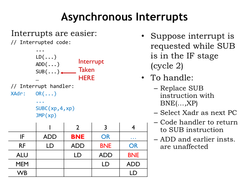
External interrupts also behave as implicit branches, but it turns out they are a bit easier to handle in our pipeline. We’ll treat external interrupts as if they were an exception that affected the IF stage. Let’s assume the external interrupt occurs in cycle 2. This means that the SUB instruction will be replaced by our magic BNE to capture the PC+4 value and we’ll force the next PC to be the address of the interrupt handler. After the interrupt handler completes, we’ll want to resume execution of the interrupted program at the SUB instruction, so we’ll code the handler to correct the value saved in the XP register so that it points to the SUB instruction.
This is all shown in the pipeline diagram. Note that the ADD, LD, and other instructions that came before SUB in the program are unaffected by the interrupt.
We can use the existing instruction-path muxes to deal with interrupts, since we’re treating them as IF-stage exceptions. We simply have to adjust the logic for IRSrc_IF to also make it 1 when an interrupt is requested.
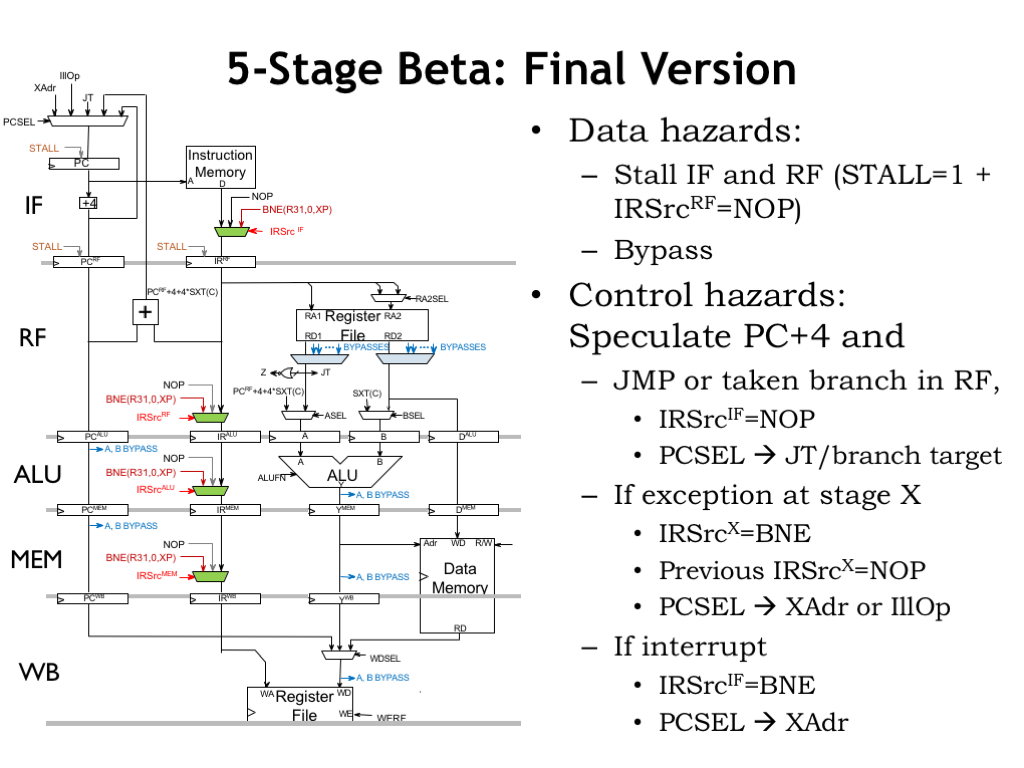
So here’s the final version of our 5-stage pipelined data path.
To deal with data hazards we’ve added stall logic to the IF and RF input registers. We’ve also added bypass muxes on the output of the register file read ports so we can route values from later in the data path if we need to access a register value that’s been computed but not yet written to the register file. We also made a provision to insert NOPs into the pipeline after the RF stage if the IF and RF stages are stalled.
To deal with control hazards, we speculate that the next instruction is at PC+4. But for JMPs and taken branches, that guess is wrong so we added a provision for annulling the instruction in the IF stage.
To deal with exceptions and interrupts we added instruction muxes in all but the final pipeline stage. An instruction that causes an exception is replaced by our magic BNE instruction to capture its PC+4 value. And instructions in earlier stages are annulled.
All this extra circuitry has been added to ensure that pipelined execution gives the same result as unpipelined execution. The use of bypassing and branch prediction ensures that data and control hazards have only a small negative impact on the effective CPI. This means that the much shorter clock period translates to a large increase in instruction throughput.

It’s worth remembering the strategies we used to deal with hazards: stalling, bypassing and speculation. Most execution issues can be dealt with using one of these strategies, so keep these in mind if you ever need to design a high-performance pipelined system.
This completes our discussion of pipelining. We’ll explore other avenues to higher processor performance in a later lecture discussing parallel processing.


