Study Materials

Course Info

Instructor

Prof. R. Rosales

Departments

Mathematics

As Taught In

Fall 1999

Level

Undergraduate

Topics

Mathematics

Learning Resource Types

Exams with Solutions

Problem Sets with Solutions

Download Course

Newton Iterations

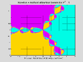
Figure 1 illustrates the complicated patterns of convergence that Newton’s method for finding roots can have. Here we have plotted the basins of attraction for the three cubic roots of unity under iterations using Newton’s method. Each color corresponds to a root. Notice how complicated the boundary between the regions is!

In fact, the boundary has a self-similar fractal structure: any piece of it that is blown up will display the whole pattern.

(All images created with MATLAB® software)

Click on picture for more information and an image of higher resolution.

Riemann Surfaces

(All images created with MATLAB® software)

Click on pictures for more information and an image of higher resolution.

One way to get a single valued function out of a multiple valued function is to introduce branch cuts in the complex plane. These are curves joining the branch points in such a way as to prevent multiple values from arising (by eliminating paths that can go around the branch points). Then a single value can be selected (at each point in the cut plane) for the function. This then defines a branch of the multiple valued function.

We point out that the process by which a branch of a multiple valued function is constructed is somewhat arbitrary; the selection of the branch cuts is only limited by the fact that they must be there to prevent the multiple values from arising. This leaves a large amount of freedom in their selection. Thus, the branches of a multiple valued function are highly non-unique and (generally) there is nothing to make one branch special over another (excepting special reasons that may arise in specific applications and uses of complex variables).

Figure 1: Real part of the Principal Value of the cube root.

Unfortunately, a price must be paid for the single valued function a branch of a multiple valued function provides. The price is that branches are discontinuous along the branch cuts. On the other hand, branches are necessary, since they provide the only practical way of actually doing computations that involve multiple valued complex functions.

We illustrate these points with the example of the principal value of the cubic root on the complex plane. This principal value is defined by the following facts: the branch cut is the negative real axis and the branch takes positive real values on the positive real axis. Equivalently, the argument of the cubic root is restricted to the range: -π/3 < θ < π/3. Figure 1 shows the real part of the principal value of the cubic root and Figure 2 shows the imaginary part. The discontinuity along the negative real axis (the branch cut) is quite evident.

Notice that, since this function can take only three values, on the complex plane cut as described here (along the negative real axis) only three possible branches can be defined. One is the principal value and the other two are just the principal value multiplied by one of the cubic roots of unity distinct from one; that is, multiplied by either: e^i2π/3 or e^-i2π/3

Furthermore, if we attempt to continue the function across the cut in a smooth fashion, the function (instead of taking the values given by the principal value) takes the values given by one of the other branches. This is a quite general phenomena: Any given branch of multiple valued function connects smoothly with some other branch when a path crossing a branch cut is followed. Here, as we cross the negative real axis, we will connect with one or the other of the two other branches, depending on which direction the crossing is made. In examples with many branch cuts and many possible branches, the situation can become quite confusing (the famous Minotaur labyrinth of Greek mythology might look trivial by comparison with the situations that relatively simple complex functions give rise to).

Figure 2: Imaginary part of the Principal Value of the cube root.

(All images created with MATLAB® software)

Figure 2: Imaginary part of the Principal Value of the cube root.

Imaginary part of the Principal Part branch of the cubic root function on the complex plane. Notice the discontinuity along the negative real axis (the branch cut).

Picture obtained using the script PlotCube in the Athena 18.04 MATLAB® Toolkit.

(All images created with MATLAB® software)

Figure 1: Real part of the Principal Vale of the cube root.

Real part of the Principal Part branch of the cubic root function on the complex plane. Notice the lack of smoothness along the negative real axis (the branch cut), where the surface has a corner.

Picture obtained using the script PlotCube in the Athena 18.04 MATLAB® Toolkit.

(All images created with MATLAB® software.)

Click on pictures for more information and an image of higher resolution.

Multiple values are impossible to avoid in the context of complex valued functions. It is a feature present even in some of the most elementary functions (such as the logarithm and the square root). Actually, multiple valued functions in the complex plane give rise to many interesting and intriguing phenomena, so perhaps the fact that they cannot be avoided is a blessing in disguise. Multiple values, of course, also arise for real valued functions. But there, quite often, the various values can be cleanly separated into different functions. Thus, one talks of the positive (or the negative) square root and the idea of the logarithm as multiple valued does not even arise!

By contrast, for functions of a complex variable, the various values are usually smoothly “connected”. By moving around in the complex plane and tracking the values of the function, it is possible to switch values after going around a closed path. Thus, it is not possible to split (in some natural/obvious way) the multiple values into different functions. The points around which these connections occur (i.e. where the value of the function switches) are called branch points.

Figure 1: Real part of the cube root on the complex plane.

We illustrate this behavior here with the example of the cubic root function on the complex plane. Figure 1 shows the real part of the cubic root and Figure 2 shows the imaginary part. At each point in the complex plane (except for the origin) there are three possible cubic roots and this gives rise to the “three level surfaces” that show in each of the pictures. But these three surfaces are, in fact, not disjoint. Notice how they wrap around the origin (a branch point) so that it is possible to go from one sheet to another simply by moving around the origin.

In fact, the three surfaces are just one nice smooth surface (except at the origin), but to see this we would have to be able to make four dimensional graphs! The crossings that occur in the pictures are similar to the crossings one would see when projecting a perfectly fine single valued curve in three dimensions with (say) a knot, onto the plane.

All of this becomes a bit clearer using the notion of the Riemann Surface associated with a multiple valued function on the complex plane. Below we will give several examples of this idea.

Figure 2: Imaginary part of the cube root on the complex plane.

(All images created with MATLAB® software)

Figure 2: Imaginary part of the cube root on the complex plane

Imaginary part of the cubic root function on the complex plane. Notice how the three levels of the surface join at the branch point at the origin. Notice also that the other crossings of levels occur in different places for the real and the imaginary parts. Thus, for the full surface of values of the function (i.e.: the surface in four dimensions given by the mapping from z to z^1/3), the only point where the levels touch is the origin.

Picture obtained using the script PlotCube in the Athena 18.04 MATLAB® Toolkit.

Figure 2: Imaginary part of the cube root on the complex plane

(All images created with MATLAB® software)

Figure 1: Real part of the cube root on the complex plane

Real part of the cubic root function on the complex plane. Notice how the three levels of the surface join at the branch point at the origin. Notice also that the other crossings of levels occur in different places for the real and the imaginary parts. Thus, for the full surface of values of the function (i.e.: the surface in four dimensions given by the map z to z^1/3), the only point where the levels touch is the origin.

Picture obtained using the script PlotCube in the Athena 18.04 MATLAB® Toolkit.

Figure 1: Real part of the cube root on the complex plane

(All images created with MATLAB® software)

Figure 1: Newton’s method of attraction basins for z3= 1.

Basins of attraction for the three cubic roots of unity under iterations using Newton’s method. Each color in Figure 1 corresponds to a root. The complicated boundary between the regions has a self-similar fractal structure: any piece of it that is blown up will display the whole pattern.

Picture obtained using the script NewtonRoots in the Athena 18.04 MATLAB® Toolkit.

Figure 1: Newton’s method of attraction basins for z³=1.

(All images created with MATLAB® software)

Click on pictures for more information and an image of higher resolution.

Figure 1: Side view of the Riemann Surface for the function f(z)=(z²-1)^1/2

To construct the Riemann Surface for the function f(z)=(z²-1)^1/2 we start with the complex plane with two cuts along the real axis: one for x > 1 and the other for x < -1. On this cut plane the function has two branches. Figures 1 & 2 illustrate these branches, which must then be joined (as usual) along the cuts to produce the Riemann Surface. The colors in the pictures are set up to be consistent with the way the branches are to be joined (red to red and blue to blue) along the lips of the branch cuts. Again, as in the case of the the square root, we must go into the “fourth dimension” to do so.

Figure 2: Another Side view of the Riemann Surface for the function f(z)=(z²-1)^1/2

That is: the Riemann Surface for f(z)=(z²-1)^1/2 is an object in four dimensional space. This surface is shown on Figure 3, where the color coding is the same as that used for Figures 1 & 2 (“Lego” blocks). Notice that Figure 3 is rotated by 90 degrees on the complex plane, relative to the first two figures.

Figure 3: Top view of the Riemann Surface for the function f(z)=(z²-1)^1/2

(All images created with MATLAB® software)

One of the branches used in the construction of the Riemann Surface for (z²-1)^1/2. The surface produced by this branch (shown here) must be joined with the surface produced by the other branch (which is just the negative of this one) along the discontinuities on the branch cuts, to produce the desired Riemann Surface.

Picture obtained using the script RiemannSur in the Athena 18.04 MATLAB® Toolkit.

Figure 1: Side view of the Riemann Surface for the function f(z)=(z²-1)^1/2

(All images created with MATLAB® software)

Picture obtained using the script RiemannSur in the Athena 18.04 MATLAB® Toolkit.

Figure 2: Another Side view of the Riemann Surface for the function f(z)=(z²-1)^1/2

(All images created with MATLAB® software)

Riemann Surface for (z²-1)^1/2. This surface is an object in four dimensions and cannot be drawn properly in three dimensions. The self intersections that the picture shows are a by-product of projecting the surface on three dimensions. The singularities in the surface are at the branch points, namely: at z=1 and at z=-1.

Picture obtained using the script RiemannSur in the Athena 18.04 MATLAB® Toolkit.

Figure 3: Top view of the Riemann Surface for the function f(z)=(z²-1)^1/2

(All images created with MATLAB® software)

Click on pictures for more information and an image of higher resolution.

Figure 1: Riemann Surface of the function f(z)=log((z+1)/(z-1))

To construct the Riemann Surface for the function f(z)=log((z+1)/(z-1)), we start with the complex plane with a single cut on the real axis (from x = -1 to x = 1), where the function has infinitely many branches. Then we proceed in the same fashion used in the previous examples. The two pictures show two views of the resulting surface.

Figure 2: Top view for the Riemann Surface of the function f(z)=log((z+1)/(z-1))

(All images created with MATLAB® software)

Riemann Surface for f(z) = log((z+1)/(z-1)). The picture shows only four levels of the surface, which extends up and down with infinitely many similar levels (notice the similarity with a parking building, with connecting ramps between levels at the center). The only singularities in the surface are at the branch points: z=1 and z=-1 (the edges of of the connecting ramps in the parking building analogy).

Picture obtained using the script RiemannSur in the Athena 18.04 MATLAB® Toolkit.

Figure 1: Riemann Surface of the function f(z)=log((z+1)/(z-1))

(All images created with MATLAB® software)

Picture obtained using the script RiemannSur in the Athena 18.04 MATLAB® Toolkit.

Figure 2: Top view for the Riemann Surface of the function f(z)=log((z+1)/(z-1))

(All images created with MATLAB® software)

Click on pictures for more information and an image of higher resolution.

Figure 1: Riemann Surface for the function f(z)=log(1-z^1/2)

The Riemann Surface for the function f(z)=log(1-z^1/2) has a new feature not seen in any of the prior cases. Namely, in this case the branch points are z=0, z=1 and infinity. However, the branch point at z=1 is peculiar, since it is a branch point only when we take the value of z^1/2 as 1 for z=1 and it is not when we take this value to be -1. This means that there are two distinct cut complex planes that one must use in constructing the surface. The first cut plane could be taken as the plane with two cuts on the real axis (on x < 0 and on x > 1) and corresponds to the case when z=1 is a branch point. There are infinitely many branches of the function on this cut plane, with their values differing by multiples of 2πi (depending on which branch of the logarithm one uses). Two views of the resulting typical “Lego” surface block are shown in Figures 1 & 2. To construct the Riemann Surface, we begin by taking infinitely many copies of this “Lego” block, stacking them one on top of the other and joining them across the matching edges of the branch cuts on x > 1 (in the pictures these edges are marked by thick lines in blue and red — the joining is then done blue in one block to red in the next one). After this first step, we end up with a surface that is somewhat similar to the spiral staircase-like Riemann Surface that the logarithm function has, except for a “small” detail: at each level in the staircase, there is a gap left by the two lips of the branch cut on the negative real axis (marked in thick magenta and green lines in the pictures).

Figure 2: Riemann Surface for the function f(z)=log(1-z^1/2)

To fill the gaps left in the surface after the first construction step described in the prior paragraph, we make use of the second cut plane, which has a single cut (on the negative real axis) and corresponds to the case when z=1 is not a branch point. Again, there are infinitely many branches of the function on this cut plane, with their values differing by multiples of 2πi. A view of the resulting typical “Lego” surface block is shown on Figure 3. We can now use these blocks to fill in the gaps left in the prior step, by joining the appropriate edges of the cuts on the negative real axis (magenta to magenta and green to green) of the two types of “Lego” blocks we have. Notice that this last step can only be done by going into a fourth dimension (to avoid crossings of the surfaces). Thus the Riemann Surface for f(z)=log(1-z^1/2) is an object in four dimensional space. We have not attempted to provide a three dimensional projection/view of this surface, but we hope that the description above gives some idea of its structure.

Figure 3: Surface generated by one of the branches where z=1 is not a branch point of f(z)=log(1-z^1/2).

(All images created with MATLAB® software)

Surface generated by one of the branches where z=1 is a branch point of f(z)=log(1-z^1/2). The other branches differ from this one by a multiple of 2πi and they give rise to infinitely many copies of this surface. To construct the Riemann Surface for f=f(z) we first stack (one on top of another) infinitely many copies of this surface.

Then we join them along the corresponding lips of the branch cuts on x > 1 (marked with thick red and blues lines on the figure) matching colors (red to blue on the next surface). This process leaves a gap at each level (due to the cut on x < 0, whose edges are marked by the magenta and green lines on the picture). These gaps are filled using the surfaces generated by the branches of f=f(z) that do not have z=1 as a branch point.

Picture obtained using the script RiemannSur in the Athena 18.04 MATLAB® Toolkit.

Figure 1: Riemann Surface for the function f(z)=log(1-z^1/2)

(All images created with MATLAB® software)

Picture obtained using the script RiemannSur in the Athena 18.04 MATLAB® Toolkit.

Figure 2: Riemann Surface for the function f(z)=log(1-z^1/2)

(All images created with MATLAB® software)

Surface generated by one of the branches where z=1 is not a branch point of f(z)=log(1-z^1/2). The other branches differ from this one by a multiple of 2πi and they give rise to infinitely many copies of this surface.

These surfaces are used (in the construction of the Riemann Surface for f=f(z)) to close the gaps left when joining the surfaces given by the branches where z=1 is a branch point. The gaps are closed by matching colors (green to green and magenta to magenta) when joining the lips of the branch cut on the negative real axis. Notice that this last step must be done by going into the fourth dimension. Thus, the Riemann surface for f(z) is an object in four dimensional space.

Picture obtained using the script RiemannSur in the Athena 18.04 MATLAB® Toolkit.

Figure 3: Surface generated by one of the branches where z=1 is not a branch point of f(z)=log(1-z^1/2).

(All images created with MATLAB® software)

Click on pictures for more information and an image of higher resolution.

Figure 1: Riemann Surface of the function f(z)=log(z²-1)

To construct the Riemann Surface for the function f(z)=log(z²-1), we start with the complex plane with two cuts along the real axis: one for x > 1 and the other for x < -1. Here the function has infinitely many branches. Then we proceed in the same fashion used in the previous examples. The two pictures show two views of the resulting surface. We note that this Riemann Surface is an object in three dimensional space. Furthermore, this is an example with three branch points, in which it differs from all the prior examples (which only had two branch points). The branch points are z=1, z=2 and infinity.

Figure 2: Top view for the Riemann Surface of the function f(z)=log(z²-1)

(All images created with MATLAB® software)

Riemann Surface for f(z)=log(z²-1). The picture shows only three levels of the surface, which extends up and down with infinitely many similar levels (again, notice the similarity with a parking building). This is an example with three branch points, which are at: z=1, z=-1 and infinity (in all the prior examples there were only two branch points). Geometrically, using the analogy with a parking building, we note that here the connecting ramps are actually two, one going from infinity to z=-1 and the other from z=1 to infinity.

Picture obtained using the script RiemannSur in the Athena 18.04 MATLAB® Toolkit.

Figure 1: Riemann Surface of the function f(z)=log(z²-1)

(All images created with MATLAB® software)

Picture obtained using the script RiemannSur in the Athena 18.04 MATLAB® Toolkit.

Figure 2: Top view for the Riemann Surface of the function f(z)=log(z²-1)

(All images created with MATLAB® software)

Click on picture for more information and an image of higher resolution.

Riemann Surfaces provide a nice way to visualize multiple valued functions in the complex plane. In fact: on its Riemann Surface a multiple valued function is single valued, it is only when the Riemann Surface is projected on the Complex Plane that the multiple values arise. However: what is the Riemann Surface for a multiple valued function and how is it defined? We will not even attempt to be rigorous here, but just give the general idea (followed by several examples). It goes as follows:

Consider a multiple valued function and all it’s branches (corresponding to some fixed set of cuts). Think of all these branches as sort of “Lego” set with which the surface will be constructed. As we pointed out earlier, these various branches will be linked: when a branch cut is approached and crossed in one of them, the natural continuation of the values of the function will correspond to some other branch. Thus, we can take all the various copies of the cut complex planes on which the branches are defined (as single valued functions) and then “join” them across the cuts according to their correspondences (each “lip” of a cut will go to a different branch). This will then produce a surface on which the function is defined as single valued in a smooth way (no discontinuities anywhere). This surface is the Riemann Surface.

For example, in the case of the logarithm, we can start with the complex plane cut along the negative real axis. On this cut plane, the logarithm has infinitely many branches, each differing from the “next” by 2πι. Thus, if we join all these cut planes (lower lip of the cut^(*1) in a plane to the upper lip of the cut in the prior plane), what we obtain is the infinite spiral staircase-like surface displayed on the picture.

Notice that the only singularity in this surface occurs at the location of the branch point. This is a general feature of Riemann Surfaces.

^(*1) By lower lip and upper lip, we mean here the sides of the cut along the negative real axis that correspond to a negative (respectively, positive) imaginary part.

Figure 1: Riemann Surface: The Logarithm

(All images created with MATLAB® software)

Infinite spiral staircase-like Riemann Surface for the logarithm. The picture shows only three levels of the surface, which extends up and down with infinitely many similar levels (all joined at the branch point at the origin).

Picture obtained using the script RiemannSur in the Athena 18.04 MATLAB® Toolkit.

(All images created with MATLAB® software)

Click on picture for more information and an image of higher resolution.

The square root provides another simple example of a Riemann Surface. The pictures here show two views of this surface, whose construction is explained next.

Consider again a Complex Plane cut along the negative real axis, just as in the case of the logarithm. However: instead of having infinitely many possible branches on this cut plane, we have now only two. These are given by the principal value of the square root and its negative (the principal value of the square root is defined in exactly the same fashion as the principal value of the cubic root was defined earlier). It would seem that this should lead to a surface simpler than that of the logarithm, but it actually does not.

Figure 1: One view of a square root Riemann Surface

The reason is as follows: when joining the two cut planes to make the surface, we have to join the lower lip of the cut in one plane with the upper in the other (and conversely). But this cannot be done within three dimensional space, since once we join one pair of lips, the members of the other pair end up on different sides of the surface. To join this second pair, we must go into the “fourth dimension” (this is exactly the same sort of difficulty you would find if you try to make a knot in a curve while staying on a plane). What this all means is that: the Riemann Surface for the square root is an object in four dimensional space. In the pictures we have color coded the surface: at the (inevitable in three dimensions) crossings each of the two sheets that cross have a clearly distinct coloring (this is the best we could do with our 4-D coloring pens broken).

Figure 2: Another view of a square root Riemann Surface

(All images created with MATLAB® software

Riemann Surface for the square root. This surface is an object in four dimensions and cannot be drawn properly in three dimensions. The self intersections that the picture shows are a by-product of projecting the surface on three dimensions. The only singularity in the surface arises at the origin (the branch point).

Picture obtained using the script RiemannSur in the Athena 18.04 MATLAB® Toolkit.

Figure 1: One view of a square root Riemann Surface