
Video 5: K-Means Clustering
Scree Plots
While dendrograms can be used to select the final number of clusters for Hierarchical Clustering, we can’t use dendrograms for k-means clustering. However, there are several other ways that the number of clusters can be selected. One common way to select the number of clusters is by using a scree plot, which works for any clustering algorithm.
A standard scree plot has the number of clusters on the x-axis, and the sum of the within-cluster sum of squares on the y-axis. The within-cluster sum of squares for a cluster is the sum, across all points in the cluster, of the squared distance between each point and the centroid of the cluster. We ideally want very small within-cluster sum of squares, since this means that the points are all very close to their centroid.
To create the scree plot, the clustering algorithm is run with a range of values for the number of clusters. For each number of clusters, the within-cluster sum of squares can easily be extracted when using k-means clustering. For example, suppose that we want to cluster the MRI image from this video into two clusters. We can first run the k-means algorithm with two clusters:
KMC2 = kmeans(healthyVector, centers = 2, iter.max = 1000)
Then, the within-cluster sum of squares is just an element of KMC2:
KMC2$withinss
This gives a vector of the within-cluster sum of squares for each cluster (in this case, there should be two numbers).
Now suppose we want to determine the best number of clusters for this dataset. We would first repeat the kmeans function call above with centers = 3, centers = 4, etc. to create KMC3, KMC4, and so on. Then, we could generate the following plot:
NumClusters = seq(2,10,1)
SumWithinss = c(sum(KMC2$withinss), sum(KMC3$withinss), sum(KMC4$withinss), sum(KMC5$withinss), sum(KMC6$withinss), sum(KMC7$withinss), sum(KMC8$withinss), sum(KMC9$withinss), sum(KMC10$withinss))
plot(NumClusters, SumWithinss, type=“b”)
The plot looks like this (the type=“b” argument just told the plot command to give us points and lines):
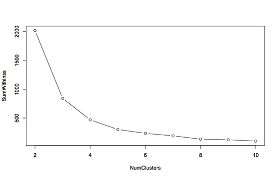
To determine the best number of clusters using this plot, we want to look for a bend, or elbow, in the plot. This means that we want to find the number of clusters for which increasing the number of clusters further does not significantly help to reduce the within-cluster sum of squares. For this particular dataset, it looks like 4 or 5 clusters is a good choice. Beyond 5, increasing the number of clusters does not really reduce the within-cluster sum of squares too much.
Note: You may have noticed it took a lot of typing to generate SumWithinss; this is because we limited ourselves to R functions we’ve learned so far in the course. In fact, R has powerful functions for repeating tasks with a different input (in this case running kmeans with different cluster sizes). For instance, we could generate SumWithinss with:
SumWithinss = sapply(2:10, function(x) sum(kmeans(healthyVector, centers=x, iter.max=1000)$withinss))
We won’t be teaching more advanced R functions like sapply in this course, but if you’re interested you could read more at the R-bloggers website.


