
Quick Question
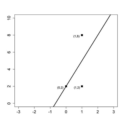
The following figure shows three data points and the best fit line
( y = 3x + 2 . )
The x-coordinate, or “x”, is our independent variable and the y-coordinate, or “y”, is our dependent variable.
Please answer the following questions using this figure.
What is the baseline prediction?
Exercise 1
Numerical Response
Explanation
The baseline prediction is the average value of the dependent variable. Since our dependent variable takes values 2, 2, and 8 in our data set, the average is (2+2+8)/3 = 4.
What is the Sum of Squared Errors (SSE) ?
Exercise 2
Numerical Response
Explanation
The SSE is computed by summing the squared errors between the actual values and our predictions. For each value of the independent variable (x), our best fit line makes the following predictions:
If x = 0, y = 3(0) + 2 = 2,
If x = 1, y = 3(1) + 2 = 5.
Thus we make an error of 0 for the data point (0,2), an error of 3 for the data point (1,2), and an error of 3 for the data point (1,8). So we have
SSE = 0² + 3² + 3² = 18.
What is the Total Sum of Squares (SST) ?
Exercise 3
Numerical Response
Explanation
The SST is computed by summing the squared errors between the actual values and the baseline prediction. From the first question, we computed the baseline prediction to be 4. Thus the SST is:
SST = (2 - 4)² + (2 - 4)² + (8 - 4)² = 24.
What is the R² of the model?
Exercise 4
Numerical Response
Explanation
The R² formula is:
R² = 1 - SSE/SST
Thus using our answers to the previous questions, we have that
R² = 1 - 18/24 = 0.25.
CheckShow Answer


