The Analytics Edge

5.5 Assignment 5

Automating Reviews in Medicine

The medical literature is enormous. Pubmed, a database of medical publications maintained by the U.S. National Library of Medicine, has indexed over 23 million medical publications. Further, the rate of medical publication has increased over time, and now there are nearly 1 million new publications in the field each year, or more than one per minute.

The large size and fast-changing nature of the medical literature has increased the need for reviews, which search databases like Pubmed for papers on a particular topic and then report results from the papers found. While such reviews are often performed manually, with multiple people reviewing each search result, this is tedious and time consuming. In this problem, we will see how text analytics can be used to automate the process of information retrieval.

The dataset consists of the titles (variable title) and abstracts (variable abstract) of papers retrieved in a Pubmed search. Each search result is labeled with whether the paper is a clinical trial testing a drug therapy for cancer (variable trial). These labels were obtained by two people reviewing each search result and accessing the actual paper if necessary, as part of a literature review of clinical trials testing drug therapies for advanced and metastatic breast cancer.

 

Problem 1.1 - Loading the Data

Load clinical_trial (CSV - 2.9MB) into a data frame called trials (remembering to add the argument stringsAsFactors=FALSE), and investigate the data frame with summary() and str().

Important Note: Some students have been getting errors like “invalid multibyte string” when performing certain parts of this homework question. If this is happening to you, use the argument fileEncoding=“latin1” when reading in the file with read.csv. This should cause those errors to go away.

We can use R’s string functions to learn more about the titles and abstracts of the located papers. The nchar() function counts the number of characters in a piece of text. Using the nchar() function on the variables in the data frame, answer the following questions:

How many characters are there in the longest abstract? (Longest here is defined as the abstract with the largest number of characters.)

Exercise 1

 Numerical Response 

 

Explanation

You can load the data set into R with the following command:

trials = read.csv(“clinical_trial.csv”, stringsAsFactors=FALSE)

From summary(nchar(trials$abstract)) or max(nchar(trials$abstract)), we can read the maximum length.

CheckShow Answer

Problem 1.2 - Loading the Data

How many search results provided no abstract? (HINT: A search result provided no abstract if the number of characters in the abstract field is zero.)

Exercise 2

 Numerical Response 

 

Explanation

From table(nchar(trials$abstract) == 0) or sum(nchar(trials$abstract) == 0), we can find the number of missing abstracts.

CheckShow Answer

Problem 1.3 - Loading the Data

Find the observation with the minimum number of characters in the title (the variable “title”) out of all of the observations in this dataset. What is the text of the title of this article? Include capitalization and punctuation in your response, but don’t include the quotes.

Exercise 3

 Text Response  Answer:A decade of letrozole: FACE.

Explanation

To identify which title is the shortest, we can use

which.min(nchar(trials$title))

From this, we know the 1258th title is the shortest. We can access this title with trials$title[1258].

CheckShow Answer

Problem 2.1 - Preparing the Corpus

Because we have both title and abstract information for trials, we need to build two corpera instead of one. Name them corpusTitle and corpusAbstract.

Following the commands from lecture, perform the following tasks (you might need to load the “tm” package first if it isn’t already loaded). Make sure to perform them in this order.

1. Convert the title variable to corpusTitle and the abstract variable to corpusAbstract.

2. Convert corpusTitle and corpusAbstract to lowercase. After performing this step, remember to run the lines:

corpusTitle = tm_map(corpusTitle, PlainTextDocument)

corpusAbstract = tm_map(corpusAbstract, PlainTextDocument)

3. Remove the punctuation in corpusTitle and corpusAbstract.

4. Remove the English language stop words from corpusTitle and corpusAbstract.

5. Stem the words in corpusTitle and corpusAbstract (each stemming might take a few minutes).

6. Build a document term matrix called dtmTitle from corpusTitle and dtmAbstract from corpusAbstract.

7. Limit dtmTitle and dtmAbstract to terms with sparseness of at most 95% (aka terms that appear in at least 5% of documents).

8. Convert dtmTitle and dtmAbstract to data frames (keep the names dtmTitle and dtmAbstract).

If the code length(stopwords(“english”)) does not return 174 for you, then please run the line of code in stopwords (TXT) file, which will store the standard stop words in a variable called sw. When removing stop words, use tm_map(corpusTitle, removeWords, sw) and tm_map(corpusAbstract, removeWords, sw) instead of tm_map(corpusTitle, removeWords, stopwords(“english”)) and tm_map(corpusAbstract, removeWords, stopwords(“english”)).

Explanation

Below we provide the code for corpusTitle; only minor modifications are needed to build corpusAbstract.

corpusTitle = Corpus(VectorSource(trials$title))

corpusTitle = tm_map(corpusTitle, tolower)

corpusTitle = tm_map(corpusTitle, PlainTextDocument)

corpusTitle = tm_map(corpusTitle, removePunctuation)

corpusTitle = tm_map(corpusTitle, removeWords, stopwords(“english”))

corpusTitle = tm_map(corpusTitle, stemDocument)

dtmTitle = DocumentTermMatrix(corpusTitle)

dtmTitle = removeSparseTerms(dtmTitle, 0.95)

¨C87C

How many terms remain in dtmTitle after removing sparse terms (aka how many columns does it have)?

Exercise 4

 Numerical Response 

 

How many terms remain in dtmAbstract?

Exercise 5

 Numerical Response 

 

Explanation

These can be read from str(dtmTitle) and str(dtmAbstract). Other than str(), the dim() or ncol() functions could have been used. If you used fileEncoding=“latin1” when reading in the datafile, you’ll have a few extra terms in dtmAbstract, but you should get the answer correct.

CheckShow Answer

Problem 2.2 - Preparing the Corpus

What is the most likely reason why dtmAbstract has so many more terms than dtmTitle?

Exercise 6

 Abstracts tend to have many more words than titles 

 Abstracts tend to have a much wider vocabulary than titles 

 More papers have abstracts than titles 

Explanation

Because titles are so short, a word needs to be very common to appear in 5% of titles. Because abstracts have many more words, a word can be much less common and still appear in 5% of abstracts.

While abstracts may have wider vocabulary, this is a secondary effect. As we saw in the previous subsection, all papers have titles, but not all have abstracts.

CheckShow Answer

Problem 2.3 - Preparing the Corpus

What is the most frequent word stem across all the abstracts? Hint: you can use colSums() to compute the frequency of a word across all the abstracts.

Exercise 7

 Text Response  Answer:patient

Explanation

We can compute the column sums and then identify the most common one with:

csAbstract = colSums(dtmAbstract)

which.max(csAbstract)

CheckShow Answer

Problem 3.1 - Building a model

We want to combine dtmTitle and dtmAbstract into a single data frame to make predictions. However, some of the variables in these data frames have the same names. To fix this issue, run the following commands:

colnames(dtmTitle) = paste0(“T”, colnames(dtmTitle))

colnames(dtmAbstract) = paste0(“A”, colnames(dtmAbstract))

What was the effect of these functions?

Exercise 8

 Removing the words that are in common between the titles and the abstracts. 

 Adding the letter T in front of all the title variable names and adding the letter A in front of all the abstract variable names. 

 Adding the letter T in front of all the title variable names that also appear in the abstract data frame, and adding an A in front of all the abstract variable names that appear in the title data frame. 

Explanation

The first line pastes a T at the beginning of each column name for dtmTitle, which are the variable names. The second line does something similar for the Abstract variables - it pastes an A at the beginning of each column name for dtmAbstract, which are the variable names.

CheckShow Answer

Problem 3.2 - Building a Model

Using cbind(), combine dtmTitle and dtmAbstract into a single data frame called dtm:

dtm = cbind(dtmTitle, dtmAbstract)

As we did in class, add the dependent variable “trial” to dtm, copying it from the original data frame called trials. How many columns are in this combined data frame?

Exercise 9

 Numerical Response 

 

Explanation

The combination can be accomplished with:

dtm = cbind(dtmTitle, dtmAbstract)

dtm$trial = trials$trial

The number of variables in the combined data frame can be read from str(dtm) or ncol(dtm). If you used fileEncoding=“latin1” when reading in the file, you should have 5 extra variables (but the answer should be graded as correct).

CheckShow Answer

Problem 3.3 - Building a Model

Now that we have prepared our data frame, it’s time to split it into a training and testing set and to build regression models. Set the random seed to 144 and use the sample.split function from the caTools package to split dtm into data frames named “train” and “test”, putting 70% of the data in the training set.

Explanation

This can be accomplished with:

set.seed(144)

spl = sample.split(dtm$trial, 0.7)

train = subset(dtm, spl == TRUE)

test = subset(dtm, spl == FALSE)

What is the accuracy of the baseline model on the training set? (Remember that the baseline model predicts the most frequent outcome in the training set for all observations.)

Exercise 10

 Numerical Response 

 

Explanation

Just as in any binary classification problem, the naive baseline always predicts the most common class. From table(train$trial), we see 730 training set results were not trials, and 572 were trials. Therefore, the naive baseline always predicts a result is not a trial, yielding accuracy of 730/(730+572).

CheckShow Answer

Problem 3.4 - Building a Model

Build a CART model called trialCART, using all the independent variables in the training set to train the model, and then plot the CART model. Just use the default parameters to build the model (don’t add a minbucket or cp value). Remember to add the method=“class” argument, since this is a classification problem.

What is the name of the first variable the model split on?

Exercise 11

 Text Response  Answer:Tphase

Explanation

This can be accomplished with:

trialCART = rpart(trial~., data=train, method=“class”)

prp(trialCART)

The first split checks whether or not Tphase is less than 0.5

CheckShow Answer

Problem 3.5 - Building a Model

Obtain the training set predictions for the model (do not yet predict on the test set). Extract the predicted probability of a result being a trial (recall that this involves not setting a type argument, and keeping only the second column of the predict output). What is the maximum predicted probability for any result?

Exercise 12

 Numerical Response 

 

Explanation

The training set predictions can be obtained and summarized with the following commands:

predTrain = predict(trialCart)[,2]

summary(predTrain)

CheckShow Answer

Problem 3.6 - Building a Model

Without running the analysis, how do you expect the maximum predicted probability to differ in the testing set?

Exercise 13

 The maximum predicted probability will likely be smaller in the testing set. 

 The maximum predicted probability will likely be exactly the same in the testing set. 

 The maximum predicted probability will likely be larger in the testing set. 

Explanation

Because the CART tree assigns the same predicted probability to each leaf node and there are a small number of leaf nodes compared to data points, we expect exactly the same maximum predicted probability.

CheckShow Answer

Problem 3.7 - Building a Model

For these questions, use a threshold probability of 0.5 to predict that an observation is a clinical trial.

What is the training set accuracy of the CART model?

Exercise 14

 Numerical Response 

 

What is the training set sensitivity of the CART model?

Exercise 15

 Numerical Response 

 

What is the training set specificity of the CART model?

Exercise 16

 Numerical Response 

 

Explanation

We can compare the predictions with threshold 0.5 to the true results in the training set with:

table(train$trial, predTrain >= 0.5)

From this, we read the following confusion matrix (rows are true outcome, columns are predicted outcomes):

FALSE TRUE

0 631 99

1 131 441

 

We conclude that the model has training set accuracy (631+441)/(631+441+99+131), sensitivity 441/(441+131) and specificity 631/(631+99).

CheckShow Answer

Problem 4.1 - Evaluating the model on the testing set

Evaluate the CART model on the testing set using the predict function and creating a vector of predicted probabilities predTest.

What is the testing set accuracy, assuming a probability threshold of 0.5 for predicting that a result is a clinical trial?

Exercise 17

 Numerical Response 

 

Explanation

The testing set predictions can be obtained and compared to the true outcomes with:

predTest = predict(trialCART, newdata=test)[,2]

table(test$trial, predTest >= 0.5)

This yields the following confusion matrix:

FALSE TRUE

0 261 52

1 83 162

 

From this, we read that the testing set accuracy is (261+162)/(261+162+83+52).

CheckShow Answer

Problem 4.2 - Evaluating the Model on the Testing Set

Using the ROCR package, what is the testing set AUC of the prediction model?

Exercise 18

 Numerical Response 

 

Explanation

The AUC can be determined using the following code:

library(ROCR)

pred = prediction(predTest, test$trial)

as.numeric(performance(pred, “auc”)@y.values)

CheckShow Answer

Part 5: Decision-maker Tradeoffs

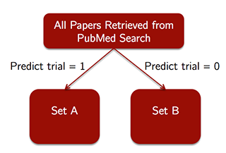
The decision maker for this problem, a researcher performing a review of the medical literature, would use a model (like the CART one we built here) in the following workflow:

1. For all of the papers retreived in the PubMed Search, predict which papers are clinical trials using the model. This yields some initial Set A of papers predicted to be trials, and some Set B of papers predicted not to be trials. (See the figure below.)

2. Then, the decision maker manually reviews all papers in Set A, verifying that each paper meets the study’s detailed inclusion criteria (for the purposes of this analysis, we assume this manual review is 100% accurate at identifying whether a paper in Set A is relevant to the study). This yields a more limited set of papers to be included in the study, which would ideally be all papers in the medical literature meeting the detailed inclusion criteria for the study.

3. Perform the study-specific analysis, using data extracted from the limited set of papers identified in step 2.

This process is shown in the figure below.

Problem 5.1 - Decision-Maker Tradeoffs

What is the cost associated with the model in Step 1 making a false negative prediction?

Exercise 19

 A paper will be mistakenly added to Set A, yielding additional work in Step 2 of the process but not affecting the quality of the results of Step 3. 

 A paper will be mistakenly added to Set A, definitely affecting the quality of the results of Step 3. 

 A paper that should have been included in Set A will be missed, affecting the quality of the results of Step 3. 

 There is no cost associated with a false negative prediction. 

Explanation

By definition, a false negative is a paper that should have been included in Set A but was missed by the model. This means a study that should have been included in Step 3 was missed, affecting the results.

CheckShow Answer

Problem 5.2 - Decision-Maker Tradeoffs

What is the cost associated with the model in Step 1 making a false positive prediction?

Exercise 20

 A paper will be mistakenly added to Set A, yielding additional work in Step 2 of the process but not affecting the quality of the results of Step 3. 

 A paper will be mistakenly added to Set A, definitely affecting the quality of the results of Step 3. 

 A paper that should have been included in Set A will be missed, affecting the quality of the results of Step 3. 

 There is no cost associated with a false positive prediction. 

Explanation

By definition, a false positive is a paper that should not have been included in Set A but that was actually included. However, because the manual review in Step 2 is assumed to be 100% effective, this extra paper will not make it into the more limited set of papers, and therefore this mistake will not affect the analysis in Step 3.

CheckShow Answer

Problem 5.3 - Decision-Maker Tradeoffs

Given the costs associated with false positives and false negatives, which of the following is most accurate?

Exercise 21

 A false positive is more costly than a false negative; the decision maker should use a probability threshold greater than 0.5 for the machine learning model. 

 A false positive is more costly than a false negative; the decision maker should use a probability threshold less than 0.5 for the machine learning model. 

 A false negative is more costly than a false positive; the decision maker should use a probability threshold greater than 0.5 for the machine learning model. 

 A false negative is more costly than a false positive; the decision maker should use a probability threshold less than 0.5 for the machine learning model. 

Explanation

A false negative might negatively affect the results of the literature review and analysis, while a false positive is a nuisance (one additional paper that needs to be manually checked). As a result, the cost of a false negative is much higher than the cost of a false positive, so much so that many studies actually use no machine learning (aka no Step 1) and have two people manually review each search result in Step 2. As always, we prefer a lower threshold in cases where false negatives are more costly than false positives, since we will make fewer negative predictions.

CheckShow Answer

Back: Detecting Vandalism on Wikipedia