2. Partial Derivatives

In this unit we will learn about derivatives of functions of several variables. Conceptually these derivatives are similar to those for functions of a single variable.

They measure rates of change.
They are used in approximation formulas.
They help identify local maxima and minima.

As you learn about partial derivatives you should keep the first point, that all derivatives measure rates of change, firmly in mind. Said differently, derivatives are limits of ratios. For example,

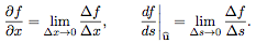
Of course, we’ll explain what the pieces of each of these ratios represent.

Although conceptually similar to derivatives of a single variable, the uses, rules and equations for multivariable derivatives can be more complicated. To help us understand and organize everything our two main tools will be the tangent approximation formula and the gradient vector.

Our main application in this unit will be solving optimization problems, that is, solving problems about finding maxima and minima. We will do this in both unconstrained and constrained settings.

Part A: Functions of Two Variables, Tangent Approximation and Optimization

» Session 24: Functions of Two Variables: Graphs
» Session 25: Level Curves and Contour Plots
» Session 26: Partial Derivatives
» Session 27: Approximation Formula
» Session 28: Optimization Problems
» Session 29: Least Squares
» Session 30: Second Derivative Test
» Session 31: Example
» Problem Set 4

Part B: Chain Rule, Gradient and Directional Derivatives

» Session 32: Total Differentials and the Chain Rule
» Session 33: Examples
» Session 34: The Chain Rule with More Variables
» Session 35: Gradient: Definition, Perpendicular to Level Curves
» Session 36: Proof
» Session 37: Example
» Session 38: Directional Derivatives
» Problem Set 5

Part C: Lagrange Multipliers and Constrained Differentials

» Session 39: Statement of Lagrange Multipliers and Example
» Session 40: Proof of Lagrange Multipliers
» Session 41: Advanced Example
» Session 42: Constrained Differentials
» Session 43: Clearer Notation
» Session 44: Example
» Problem Set 6

Exam 2

» Practice Exam
» Session 45: Review of Topics
» Session 46: Review of Problems
» Exam Materials

« Previous | Next »

» Practice Exam
» Session 45: Review of Topics
» Session 46: Review of Problems
» Exam Materials

« Previous | Next »

We start this unit by learning to visualize functions of several variables using graphs and level curves. Following this we will study partial derivatives. These will be used in the tangent approximation formula, which is one of the keys to multivariable calculus. It ties together the geometric and algebraic sides of the subject and is the higher dimensional analog of the equation for the tangent line found in single variable calculus. We will use it in part B to develop the chain rule.

We will apply our understanding of partial derivatives to solving unconstrained optimization problems. (In part C we will solve constrained optimization problems.)

» Session 24: Functions of Two Variables: Graphs
» Session 25: Level Curves and Contour Plots
» Session 26: Partial Derivatives
» Session 27: Approximation Formula
» Session 28: Optimization Problems
» Session 29: Least Squares
» Session 30: Second Derivative Test
» Session 31: Example
» Problem Set 4

« Previous | Next »

As in single variable calculus, there is a multivariable chain rule. The version with several variables is more complicated and we will use the tangent approximation and total differentials to help understand and organize it.

Also related to the tangent approximation formula is the gradient of a function. The gradient is one of the key concepts in multivariable calculus. It is a vector field, so it allows us to use vector techniques to study functions of several variables. Geometrically, it is perpendicular to the level curves or surfaces and represents the direction of most rapid change of the function. Analytically, it holds all the rate information for the function and can be used to compute the rate of change in any direction.

» Session 32: Total Differentials and the Chain Rule
» Session 33: Examples
» Session 34: The Chain Rule with More Variables
» Session 35: Gradient: Definition, Perpendicular to Level Curves
» Session 36: Proof
» Session 37: Example
» Session 38: Directional Derivatives
» Problem Set 5

« Previous | Next »

In this part we will study a new type of optimization problem: that of finding the maximum (or minimum) value of a function w = f(x, y, z) when we are only allowed to consider points (x, y, z) which are constrained to lie on a surface. The technique we will use to solve these problems is called Lagrange multipliers.

» Session 39: Statement of Lagrange Multipliers and Example
» Session 40: Proof of Lagrange Multipliers
» Session 41: Advanced Example
» Session 42: Constrained Differentials
» Session 43: Clearer Notation
» Session 44: Example
» Problem Set 6

« Previous | Next »

Browse Course Material

Course Info

Instructor

Departments

As Taught In

Level

Topics

Learning Resource Types

Multivariable Calculus