Vectorization and User-Defined Functions

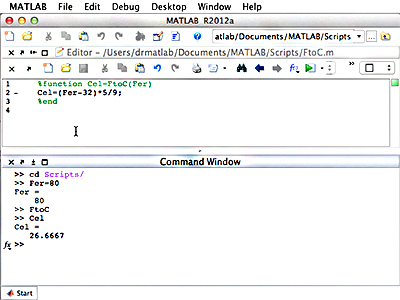
Screenshot of a function definition to convert Fahrenheit to Celsius and the respective function call.

Another convenience of MATLAB® is its ability to manipulate complex numbers, such that you can take powers and roots of any number. For practice, you will be asked to calculate and plot the basins of attraction for a polynomial in the complex plane.

Also in this unit, you will learn how to create a user-defined function in MATLAB. It is important to understand the difference between a script and a function. While a script is a separate piece of code that performs a certain task, it deals with the variables from the caller, and cannot accept input values or provide return values. Functions, on the other hand, can receive an input and deliver an output, and the variables contained therein are isolated from those of the caller. In determining whether a script or function should be used, you will need to consider the scope of the variable. Within a function, variables exist within that small space of code, and values changed within the lines of code in the function will not affect those outside in the calling workspace.

With this knowledge, your first task will be to write a function that calculates the Fibonacci numbers. This function will be recursive, meaning that it calls itself, because each Fibonacci number is calculated by taking the sum of the previous two Fibonacci numbers in the sequence.

As an exercise, you will be given a piece of code that calculates and plots the solution to the Van-der-Pol oscillator. You will also be given a series of tasks by which to edit the code and resulting plot, and later, to debug the code.

The videos below demonstrate, step-by-step, how to work with MATLAB in relevance to the topics covered in this unit.

Lecture 5: Scripts and Functions
This video includes material supplementary to Scope.
Lecture 6: Debugging
This video includes material supplementary to Scope, Homework 3.

Complex numbers $x+iy$ can be dealt with “natively” in MATLAB®. This means that you can take powers and roots of any number. One surprising and very powerful fact about complex functions is that a single derivative (not a $2\times2$ Jacobian) gives you the full derivative information (assuming that the function is analytic).

Exercise 12: Modify your 1D Newton’s method to find the basins of attraction of a interesting (degree > 3) polynomial. Plot the basin of attraction as before, but now you will have to create your initial value by $z=x+iy$. For the roots: either use a polynomial for which you know the roots, or find the roots in advance, by using your own Newton solver.

Here’s the basin of attraction of the roots of $z^5+1$:

A colorful 1000x1000 plot of basin of attraction with radial symmetry.

A plot of the basin of attraction with complex roots.

How long does it take your code to make a 1000 by 1000 plot (that is, a plot in which both the x- and y-axes have 1000 points)? If it’s more than 1 minute, your code is too slow. The reason for that is that MATLAB can be inefficient with explicit loops. In this case, we have nested loops and a plot command inside them; this is a disaster!

We need to “vectorize” the calculation and only plot once at the end after we have the result. This means instead of having MATLAB loop over the points and calculating each one at a time, you set them all up in a big matrix/vector and iterate on all of them together:

We let a matrix $A$ hold all the values of the iterations that correspond to the different points we will end up plotting. Thus we can set up the initial $A$ as follows:

N=1000;
x=linspace(-5,5,N);% linspace is another function that creates vectors.
y=linspace(-5,5,N); % Read about it!
A=ones(N,1)*x + 1i*y'*ones(1,N);

Exercise 13. Make sure you understand:

What does ones do? Find out using help ones
Can you guess what zeros does?
We can also use meshgrid for this, can you understand how to do it?

In the one-at-a-time Newton’s method the update step is

\begin{equation} \label{eq:7} x_{n+1}=x_n-\frac{f(x)}{f’(x)} \end{equation}

We want to do the same only updating all of $A$ at every step. It would work just fine if we could write

A=A-f(A)./f'(A); %Notice the ./ ? This means, POINT-WISE multiplication,
% not linear algebra

And we can. We only need to make sure that we define functions $f$ and $f’$ that know how to work with a matrix and return the right answer. We can also make our code more flexible by using our own functions ($f(x)$ and $f’(x))$. Here is how to define simple (one command) functions:

f=@(x) x.^5+1; %Notice the point here? However there's no such thing as .+
fp=@(x) 5*x.^4;

After defining f and fp, they can be used like any other MATLAB function:

>> f(1)
ans =
     2
>> f([1 2 3])
ans =
     2    33   244
>> f([1 2; 3 4])
ans =
       2          33
     244        1025

Last, but not least, plotting a 2D surface (the following code has nothing to do with our problem, but it illustrates how to plot a nice 2D surface):

x=linspace(0,2*pi);
y=x';
[X,Y]=meshgrid(x,y);%x,y are vectors,X,Y are matrices
Z=sin(X).*cos(Y.^2);
pcolor(X,Y,Z);

There are slight variations to pcolor: mesh, surf, and more. Learn about them using the help command.

Project 2. Update your Newton’s basin of attraction code to work using matrix-at-a-time update. Use pcolor to create the resulting basin plot. Your result should be much faster.

Functions define a small world of variables that are isolated from the rest of the “workspace”. This is mostly a good thing, though you may find it limiting at times. It is important to realize that a function can call itself, and even then the variables inside the called function cannot interact directly with those of the calling workspace. Here is an example to show this:

function triangle(n)
     n
     if n > 1
          triangle(n-1)
     end
     n

This is a function with no output, that calls itself. Calling it from the command-line gives:

>> triangle(4)
n =
     4
n =
     3
n =
     2
n =
     1
n =
     1
n =
     2
n =
     3
n =
     4

Exercise 14: Write a function that recursively (a function that calls itself is called recursive) calculates the Fibonacci numbers:

$$ F_1=1, \qquad F_2=1, \qquad F_{n+2}=F_{n}+F_{n+1} $$

Try it out for small value of n (it will not work for large ones). (The resulting sequence is 1, 1, 2, 3, 5, 8, 13, 21, 34, 55,….)

User-defined functions are useful in providing structure to your code. When writing code try to think in terms of functions. Separate the big task into smaller ones and define them in terms of input and output. Your main code should then be easier to read as it will consist of calls to the functions, each of which has a clearly defined task. Notice that in a function file, one can define more than one function. Simply start a new line with the keyword function and continue as before. This function will only be directly callable from within the file (since the name of the file matches a different function) though there are tricks by which one can still provide access to such “hidden” functions (too advanced for this course).

For guided practice and further exploration of scripted functions, watch Video Lecture 5: Scripts and Functions.

Here’s an example of a function that calculates and plots the solution to the Van-der-Pol oscillator (must be saved into a file called VDPDemo.m):

function VDPDemo(mu)
% solve an ODE using Runge-Kutta 4/5:
[t,X]=ode45(@dXdt,[0,100],[0;1]);

% plot the resulting phase plane trajectory:
plot(X(:,1),X(:,2))

% Here we define the derivative function.
% By nesting this function inside the main one, we get access to the
% variable mu, defined in the outer function
function dX=dXdt(t,X)
     x=X(1);
     v=X(2);

     dx=v;
     dv=-x+mu*(1-x^2)*v;

     dX=[dx;dv];
end % of dXdtg
end % of VDPDemo  

% Were the function dXdt defined here, (after the end keyword that closes
% the VDPDemo function) the variable mu would be undefined and the code
% would not run.

We can run this function by calling it with the value for mu from the command prompt:

>> VDPDemo(2)

which results in the figure:

Graph of the oscillator iterations in blue.

Plotting the solution to the Van-der-Pol oscillator.

Exercise 15: Run the Van-der-Pol oscillator several times with various input values. Observe the change in shape.

Change the code for the Van-der-Pol oscillator:

Add a green marker at the beginning of the trajectory
Add a red marker at the end of the trajectory
Plot an approximation of the “limit cycle” in black
(Bonus) find out what the period of the limit cycle is, modify the function so that it returns this value, write an additional function or script that calls VDPDemo for many values of mu and plots the dependence of the period on mu. Perhaps, to find the period of the limit cycle, you can write a function that accepts an approximation to the period of the limit cycle and returns a positive number if it’s too big and a negative number when it’s too small. you can then use this function with a secant method root finder, to find quickly the period of the limit cycle.

(Hint 1: Read the helpfile for plot carefully to understand how to change the defaults) (Hint 2: Remember that to plot several plots on the same figure without erasing the previous figure you need to issue a hold on command.)

Homework 3. Debug this code. Put a break-point on the first line in the inner function and run the code (with input 2 for example). Step over ode45 and see how you can see the values of variables by “hovering” the mouse pointer over the variable in the editor. This only works if the variable can be “seen” from the current scope. Click “step” a few times to see the code advancing.

Now terminate this execution.

Change the code so that the function dXdt is defined outside the main function (by moving one end placement). Debug again and notice how the variable mu is no longer visible inside the function dXdt. At what point does the code fail?

For guided practice and further exploration of debugging, watch Video Lecture 6: Debugging.

We have just seen—above, using the $@(x)$ notation—an example of how to create simple user-defined functions. This notation can only have one line of code, and oftentimes that can be insufficient for the task at hand. We have also seen scripts files, in which we can put many lines of code and then “call” the script to have MATLAB® execute the lines in that script. So what’s a function and how is it different from a script?

A function is also a file with lines of code, but there are several distinctions between a function and a script:

SCRIPT	FUNCTION
Interacts with variables from the caller	Has very restricted interaction with the caller
Cannot accept input	Can accept input
Cannot return a value	Can return a value
Can overwrite variables by mistake	No need to worry, variables are “local”
Cannot have “sub-functions” in file	May define more functions in same file

When we “call” a function we usually give it input and expect output. For example:


>>a=sin(pi/2)
a =
     1

We gave the input pi/2 to the function sin and assigned the output to the variable a. The function sin is not written in MATLAB code, so we cannot see how it is implemented, though on occasion it can be useful to see how some MATLAB functions are implemented. For example the function randperm(n) returns a random ordering of the numbers 1:n. It is implemented in MATLAB and can be viewed by writting open randperm (your copy of MATLAB might have a different implementation, but here’s mine):

function p = randperm(n)
%  RANDPERM Random permutation.
%    RANDPERM(n) is a random permutation of the integers from 1 to n.
%    For example, RANDPERM(6) might be [2 4 5 6 1 3].
%
%    Note that RANDPERM calls RAND and therefore changes the state of the
%    random number generator that underlies RAND, RANDI, and RANDN.  Control
%    that shared generator using RNG.
%
%    See also RNG, PERMUTE.

%    Copyright 1984-2010 The MathWorks, Inc.
%    $Revision: 1311 $  $Date: 2012-06-18 14:27:32 -0400 (Mon, 18 Jun 2012) $

[~,p] = sort(rand(1,n));

Notice that the first line starts with the keyword function, which states that this file contains a function rather than a script. Next comes the declaration of the return value p. This means that the value of the variable, p when this function terminates, will be returned as the output of the function. Next comes the name of the function. This should match the name of the file. Now the list of input variables, only one in this case: n. So whatever the input is when the function is called, internally it will be placed in a variable called n. Next there’s a long comment block which becomes the help file text (type help randsort and see) and finally the actual body of the function. In this case it is one line of code, but it is slightly strange; it turns out that you can return more than one value from a function. The function sort normally returns the inputs vector sorted:

>> sort(rand(1,4))
ans =
     0.1822    0.3957    0.4644    0.6998

But if you ask for two output variables, sort will also tell you the permutation needed to get from the input to the output:


>> A=rand(1,4)
A =
     0.9473    0.1685    0.5514    0.2684
>> [B,C]=sort(A)
B =
     0.1685    0.2684    0.5514    0.9473
C =
     2     4     3     1
>> A(C) % Notice how we use the permutation C to PERMUTE the elements of A
ans =
     0.1685    0.2684    0.5514    0.9473

As this code uses the random number generator ‘rand’, the results you get may be different from these.

As the original list of numbers is random, it implies that the permutation needed to sort it is a random, uniformly distributed permutation, and this is what MATLAB returns as the output of the function randperm. Notice the use of the tilde character to signify that the first return value isn’t needed. This is a new expansion of the MATLAB language. If you have an old version, the code will have a “throw-away” variable (a variable that is not used).

Code an arbitrary precision (integer) addition code. The start of the code should be where the “numbers” are defined. For example:

These numbers are to big to be represented exactly in MATLAB®. Your task is to write code that follows the rules of addition (adding from smallest to largest) and gets the precise answer, in the same format (that is an array of integers). There are various limitations that need to be discussed:
- First try doing this while allowing yourself only to add small 20 numbers using MATLAB +. You will still need to be crafty about how you find the “ones’’ and “tens’’ of a given number. Since MATLAB is good with lists, think how you can use a list to do this. You may not use high level functions like mod, rem etc. (But you are encouraged to familiarize yourself with them.)
- Can you do it with a matrix that represents the addition table for numbers between 0 and 11? Once you create this matrix, you can solve this exercise with +1 as the only “allowed’’ arithmetic operation (because MATLAB’s index of lists starts from 1 and not 0).
- Redo this exercise for a different definition of addition, for example, for Z₁₆.
Modify the Newton code you wrote for the basin of attraction to look at the basins for another function. How about $f(x,y)=(x^4-y, y^4-x)^T$? You will have to look for zeros (manually or otherwise) and then change your code and recalculate the Jacobian matrix.
What is $\sqrt{-1}$?
What is $(1+i)^4$?
Can you find the roots of $x^2+2x+4$?
Where are the roots of $x^5+1$?
To operate NOT in a linear algebra way on vectors, you need to put a point (.) in front of the operator: thus 1./[1 2 4] is [1 .5 .25]. Similarly with .*. Calculate $\pi$ by this really (really) bad way: For a large $N$ calculate $\sum_{n=1}^N\frac{1}{n^2}$. This converges to $\pi^2/6$ as $N\rightarrow\infty$. Calculate $\pi$ using this and find out how large $N$ must be for the resulting value of $\pi$ to be within 1e-6 of the MATLAB value pi.

N1=[1 9 5 4 3 8 4 8 5 6 0 3 4 0 5 3 2 4 5 6 ]; % to mean  19543848560340532456
N2=[2 3 4 3 2 3 4 5 4 8 6 4 7 8 9 7 6 5 3 2 1 4 6 7 9 ];

Browse Course Material

Course Info

Instructor

Departments

As Taught In

Level

Topics

Learning Resource Types

Introduction To MATLAB Programming