
Main | Hardware | System Model | Linearized Control | Nonlinear Control | Movies | Technical Details | Credits
Linearization
With the system model in hand we can turn our attention to control issues. Before a control scheme can be designed and implemented for this magnetic levitator, however, the equations of motion must be set in a form conducive to control. Unlike a mass, spring, dashpot system or an LRC circuit, the equation of motion of this levitator is nonlinear in both the input variable (i) and the state variable (x). The simplest solution to this is to linearize the equation of motion around a desired operating point, then apply traditional linear controls methods. The validity of this approach is restricted to small motions about the operating point. However, the advantages of working with a linear model mean that this technique is frequently applied in practice.
In the modeling section, the equations pertaining to the system are given as:
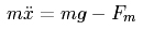
Eq. M1.
Eq. M2.
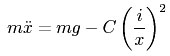
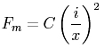
Eq. M3.
The first step in linearizing the equation is to approximate i and x as:
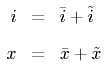
Eq. L1.
where the bar (-) is the value at the operating point, and the tilde (~) term represents incremental variations around this point. We assume  and
and  . Substituting (L1) into (M2) and taking the Taylor expansion yields:
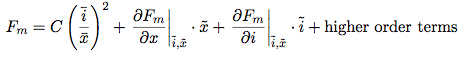
Eq. L2.
For our chosen first order aproximation, the higher order terms drop out. The two partial differential terms in the equation solve as:
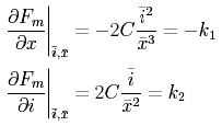
Eq. L3.
Substituting (L3) into (L2) while dropping the higher order terms leaves:
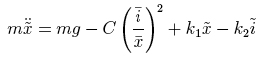
Eq. L4.
By definition, the equilibrium point is where there is no net acceleration, and where the incremental terms are equal to zero. At this point, (L4) becomes:
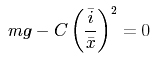
Eq. L5.
Putting (L5) into (L4) and rearranging, the equation of motion takes on the familiar form of:
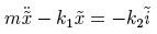
Eq. L6.
The poles of this system are at:
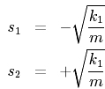
Eq. L7.
For various lengths of the airgap, the pole locations are:
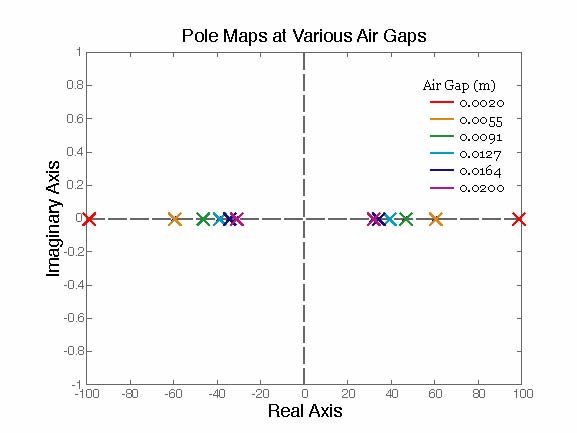
Fig. L1.
Plotting pole spacing against air gap distance results in the curve:
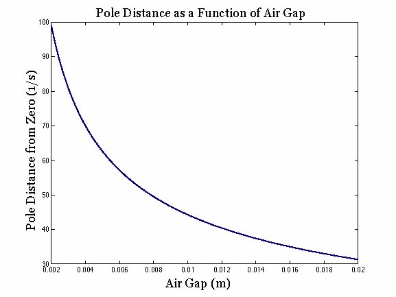
Fig. L2.
If the terms are properly expanded, the system pole locations can be shown to depend only on upon gravity and the operating air gap:
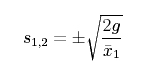
Eq. L8.
When a properly designed controller is added to an unstable system, it serves to move right-half plane poles into the left half plane. The closer the unstable pole starts to zero, the easier it is to pull it across to stability. As the above relationship between pole location and opperating point shows that pole distance from zero decreases with increasing distance between the actuator and the ball. Large distances are, however, impractical in terms of building the actuator, as the magnetic force falls off with the square of the opperating point distance, requiring a commesurate increase in current to balance the forces.
Control
Now that the system has been linearized, a controller can be applied to it. Various methods can be applied to show that a simple proportional gain controler is insufficient for this system and would not do better than to place both poles on the imaginary axis. Adding a zero to the system through the application of a proportional-differential controller can be shown by the same methods to pull the poles into the left-half plane.
The block diagram below represents the whole system. C1 represents the constant for converting between position and voltage in the position sensor and in the input. The other three blocks, from left to right, are the controller, the current supply and the plant.
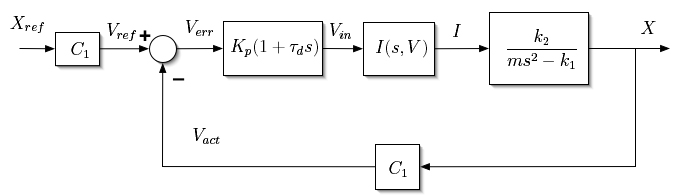
Fig. L3.
For the purposes of examining the behavior of the controlled system, it is useful to consolidate the block diagram before analyzing it. The dynamics of available current controls are sufficiently faster than those of the plant that the block can be treated as a constant multiplier and incorporated into the controller gain. C1 and k2 can be similarly incorporated. The resulting block diagram, with G representing the combination of the constant multipliers, is:
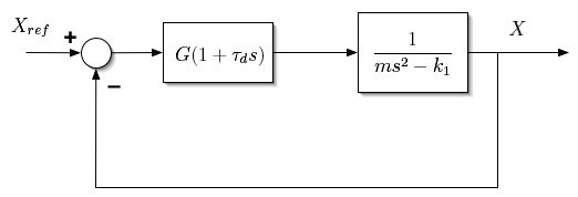
Fig. L4.
Applying Black’s Law to the simplified block diagram results in the following transfer function:
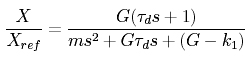
Eq. L9.
The mechanical equivalent system to the linearized model is:
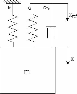
Fig. L5.
For G>k1, the system can be seen from the equation or the equivalent model to be stable. Putting the equation into cannonical form,
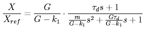
Eq. L10.
the steady state gain is seen to be K/(K-k1), which approaches unity as K gets large. Note that unlike a traditional second order system, the steady state gain here approaches unity from infinity, rather than from a fraction less than one. This effect is a result of the “negative spring” in the linearized equation of motion (Eq. L6).
Where steady state performance improves with increasing G, transient performance depends on all of the system’s characteristics. Once a value of G is chosen to provide the acceptable steady state performance, however,  is the only undefined term in the transfer function, and can be solved for to optimize transient performance.
The poles of (Eq. L9) are located at
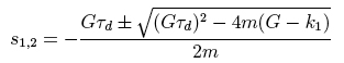
Eq. L11.
Critical damping occurs when the poles are co-located, where
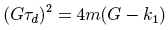
Eq. L12.
Solving for provides
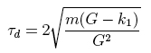
Eq. L13.
It should be noted that the controller presented above is not physically realizable, as it contains an isolated zero, which gives gain as ever increasing with frequency. A more realistic controller would have a transfer function resembling
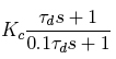
Eq. L14.


