20.109 | Spring 2010 | Undergraduate

Laboratory Fundamentals in Biological Engineering

Labs

Contents:

Lab work is divided into three modules of eight sessions each. Learning materials for each lab session (linked below under ‘Lab Materials’) include an introduction, experimental protocol, and a reagents list, followed by a “for next time” homework assignment. A short pre-lab lecture preceeds most of the lab sessions.

Selected results from some labs are included courtesy of the students and used with permission.

Lab Basics

WORKING IN THE LAB COMMUNICATING YOUR WORK

General lab policies, do’s and don’ts

Guidelines for working in the tissue culture facility

Guidelines on using personal protective equipment, developed by 
MIT’s Environmental Health and Safety Office:

Statement on Collaboration and Integrity

Guidelines for maintaining your lab notebook

Guidelines for oral presentations

Guidelines for writing up your research

First Day: Lab Orientation

There are ten stations for you and your lab partner to visit on your lab tour today. Some will be guided tours with a TA or faculty there to help you and others are self-guided, leaving you and your partner to try things on your own. Your visit to each station should last ~10-15 minutes. It doesn’t matter which station you visit first but you must visit them all before you leave today. Afterward, you should have some time remaining to begin the For Next Time assignment, and are strongly encouraged to do so. Your lab practical next time will assess your mastery of a selection of these stations - all are fair game, as is the lab safety material covered in today’s pre-lab lecture.

PRE-LAB LECTURE LAB Materials
(PDF Lab orientation

Module 1: RNA Engineering

Instructors: Jacquin Niles and Agi Stachowiak

In this module you will investigate RNA aptamer selection. You may already be familiar with peptides or proteins, such as antibodies, that bind to specific molecules. Short fragments of RNA – called RNA aptamers - can have secondary structures that also allow them to bind a target molecule with good affinity and specificity. Normally, RNA aptamers that bind particular targets are found by screening many candidates at random in a process called SELEX, or systematic evolution of ligands by exponential enrichment; however, predictive computational tools can also be used. In the coming weeks, you will essentially perform one round of SELEX. Because SELEX typically takes several rounds to isolate target-binding aptamers, you will start with a known aptamer mixture rather than than a completely random library. Your goal will be to explore what experimental parameters affect the enrichment of a heme-binding RNA aptamer from a mixture of heme-binding and non-binding RNAs.

Acknowledgement: We thank 20.109 instructor Natalie Kuldell for helpful discussions and for acquiring funding for module development.

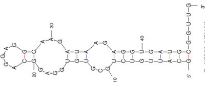
Public domain image. (Prepared using RNA Folding (mfold) at the mFold Web Server). Reference: Zuker, M. “Mfold Web Server for Nucleic Acid Folding and Hybridization Prediction.” Nucleic Acids Res. 31, no. 13 (2003): 3406-3415.

MODUle 1: RNA Engineering
LAB DAYS PRE-LAB LECTURES LAB Materials
Day 1 (PDF) Amplify aptamer-encoding DNA
Day 2 (PDF Purify aptamer-encoding DNA
Day 3 (PDF Prepare RNA by IVT
Day 4 (PDF) Purify RNA and run affinity column
Day 5 (PDF RNA to DNA by RT-PCR
Day 6 (PDF Post-selection IVT and journal club
Day 7 (PDF Aptamer binding assay
Day 8   Journal club (contd.)

See the Assignments page for descriptions of the Module 1 laboratory report and RNA computational analysis assignments.

TA notes for Module 1

Module 2: Protein Engineering

Instructors: Alan Jasanoff and Agi Stachowiak

In this experiment, you will modify a protein called inverse pericam (developed by Nagai, et al.) in order to affect its functions as a sensor. Inverse pericam (IPC) comprises a permuted fluorescent protein linked to a calcium sensor. The “inverse” in the name refers to the fact that this protein shines brightly in the absence of calcium, but dimly once calcium is added. The dissociation constant _K_D of wild-type IPC with respect to calcium is reported to be 0.2 μM (see also figure below). Your goal will be to shift this titration curve or change its steepness by altering one of the calcium binding sites in IPC’s calcium sensor portion. You will modify inverse pericam at the gene level using a process called site-directed mutagenesis, express the resultant protein in a bacterial host, and finally purify your mutant protein and assay its calcium-binding activity via fluorescence. In the course of this module, we will consider the benefits and drawbacks of different approaches to protein design, and the types of scientific investigations and applications enabled by fluorescently tagged biological molecules.

Reference: Nagai, T., et al. “Circularly Permuted Green Fluorescent Proteins Engineered to Sense Ca2+.” PNAS 98, no. 6 (March 6, 2001): 3197-3202. [Open Access]

We gratefully acknowledge 20.109 instructor Natalie Kuldell for helpful discussions during the development of this module, as well as for her prior work in developing a related module in the Spring 2007 course.

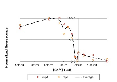
Raw titration curve for IPC. Shown here is sample data from the teaching lab: normalized fluorescence for wild-type inverse pericam as a function of calcium concentration. As you will later learn, an apparent KD can be estimated from such a plot: it is the point on the x-axis where the curve crosses y = 50%, or ~0.5 μM here

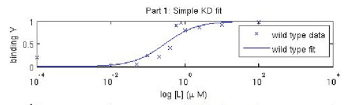
Fitted titration curve for IPC. A more sophisticated analysis using curve-fitting reveals KD to be ~ 0.3 μM, closer to the reported value for inverse pericam.

Module 2: Protein Engineering
LAB DAYS PRE-LAB LECTURES LAB Materials
Day 1 (PDF Start-up protein engineering
Day 2 (PDF) Site-directed mutagenesis
Day 3 (PDF) Bacterial amplification of DNA
Day 4 (PDF) Prepare expression system
Day 5 (PDF) Induce protein and evaluate DNA
Day 6 (PDF) Characterize protein expression
Day 7   Assay protein behavior
Day 8   Data analysis

See the Assignments page for a description of the Module 2 protein engineering research paper.

TA notes for Module 2

Module 3: Cell-Biomaterial Engineering

Instructor: Agi Stachowiak

What makes a cell become one type and not another? How can we influence this process, and why would we even want to? When faced with conflicting information – in our own experiments, or in the broader scientific literature – how do we determine what is credible? These are just some of the questions you will explore in the third and final module, all in the context of tissue engineering. The goal of tissue engineering (also called regenerative medicine) is to repair tissues damaged by acute trauma or disease. Repair is stimulated by insertion of a porous scaffold at the wound or disease site; the scaffold may carry relevant mature or progenitor cells, and in some cases also soluble growth factors. In cartilage tissue, mature cells are called chondrocytes, and their progenitor cells are mesenchymal stem cells. Tissue regeneration shares many characteristics with natural tissue development, including the importance of appropriate cell differentiation and phenotype maintenance. You will perform a hypothesis-driven investigation of the effects of environmental manipulations on primary chondrocytes and/or mesenchymal stem cells. In particular, you will assess cell viability, genotype, and protein production, but the specific experimental question is up to you.

I gratefully acknowledge Professor Alan Grodzinsky and several members of his lab group (particularly Rachel Miller and Paul Kopesky), for their technical advice and stimulating discussions during the development of this module.

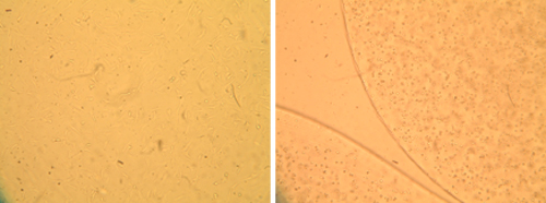
Morphology of primary bovine chondrocytes grown under two different culture conditions. Optical micrographs of chondrocytes grown in monolayer (left) and alginate bead culture (right) are shown. Cells in the 3D culture retain a round phenotype, while cells on the flat surface extend processes and spread out.

Module 3: Cell-Biomaterial Engineering
Lab DAYS PRE-LAB LECTURES LAB Materials
Day 1 (PDF) Start-up biomaterials engineering
Day 2   Initiate cell culture
Day 3 (PDF) Testing cell viability
Day 4 (PDF) Preparing cells for analysis
Day 5 (PDF) Transcript-level analysis
Day 6 (PDF) Protein-level analysis
Day 7 (PDF) Wrap-up analysis
Day 8   Student presentations

See the Assignments page for a description of the Module 3 cell-biomaterial engineering report.

TA notes for Module 3

< Previous lab day | Module 3 lab index | Next lab day >

Introduction

Last time you proposed culture conditions for an investigation of chondrocyte phenotype induction or maintenance, and today you will initiate said cultures. The chondrocyte cells you are using were freshly derived from bovine cartilage by enzymatic digestion and immediately frozen. The stem cells were grown from bovine bone marrow over the course of a few weeks, then frozen after 1-2 passages. Cells from cows are often used in part because of their availability from abattoirs. In general, large animals are more useful for modeling human joint diseases such as osteoarthritis than are small animals, because the resting angle of their knee joints is more similar to that of humans. In this module, we will work with an in vitro culture model of cartilage-forming cells.

Your two cell samples will be grown in alginate bead cultures. You have probably encountered alginates many times in your life, as thickeners in food and textiles, preservatives, and possibily at your dentist or in a pharmacy. Alginate is a polysacharride derived from seaweed, a co-polymer of mannuronic and guluronic acid. A single alginate molecule may contain long stretches of either acid (called M-blocks and G-blocks), as well as random and/or strictly alternating G/M sequences. The precise chemical composition of an alginate determines its mechanical properties, degradability, and other important characteristics. Qualities such as strength and viscosity are also influenced by the average length of the individual polymer chains (i.e., the molecular weight), and by alginate concentration. For example, high molecular weights correlate with increased viscosity. Alginates in general are shear-thinning, which is to say their viscosity decreases as shear rate increases (e.g., when quickly drawn into a syringe).

Schematic of cross-linked alginate. G-blocks are represented by dotted lines, M-blocks by curved solid lines, and calcium ions by green circles.

Cations such as calcium can cross-link alginate chains to form a network, or gel. The identity and concentration of the cross-linker influence the ultimate material properties. Only G-blocks can be linked to each other, while M- or MG-blocks cannot, but in turn provide flexibility (see figure). The resultant semi-solid structure has the capacity to hold a large amount of water, and the water-swollen structure is called a hydrogel. Hydrogels have several attractive properties for tissue engineering: they allow oxygen and nutrients to diffuse better than non-hydrated materials do; their mechanical and biochemical properties are readily varied by co-polymerization of multiple elements; they mimic the elasticity of natural tissues, and they often form rapidly and under mild conditions. Some gels can be injected into a patient in liquid form, then solidified within his or her body by heat or light. Such injectable gels have the advantage of easily filling an arbitrarily sized wound shape, which is difficult for implantable gels to do. Natural (e.g., alginate) and synthetic (e.g., poly(ethylene glycol)) hydrogels each have distinct advantages and disadvantages, as we will discuss in class.

Today you will make alginate hydrogels in bead form, by slowly releasing alginate solution from a syringe into a bath containing calcium chloride. Next time you will see how well your cells survived.

Protocols

Half the class at a time will work in the tissue culture room today. The other half of you will explore the NCBI bovine information site, and otherwise spend the time however you find useful (“For Next Time” assignment on design plan and expected assay results, notebook prep, or unrelated work).

Part 1: Chondrocyte or Stem Cell Culture

Today you will work with primary cells that are directly isolated from bovine knee joints. Recently, your teaching faculty harvested cartilage fragments from two bovine knees, and sequentially digested them in pronase and collagenase enzymes. Each joint typically yields > 50-100M cells. After cell isolation, aliquots of several million cells each were frozen and stored in liquid nitrogen.

Preparation

  1. Begin by setting up your hoods. Prepare any standard equipment and solutions needed.
  2. Note that the small beakers are for making a calcium chloride bath (not shared, one per person), and the large are for temporary waste in steps 10-12 below (shared, one per hood).
  3. If you requested a special reagent or equipment, check with the teaching faculty.
  4. If you are doing an alternative protocol (e.g., 2D culture or collagen gels), check with the teaching faculty.

Cell culture

  1. When your hood is ready, thaw your aliquot(s) of frozen cells in the water bath. Avoid immersing the cap of the tube in the bath, just hold the body submerged. Agitate the vial slightly while you hold it. The cells should thaw in less than 5 minutes.
  2. Spray the vial with 70% ethanol and take it into your hood. Using a P1000, add the cells drop-wise into the 15 mL conical containing 9 mL of pre-warmed medium. Spin at 800 g for 8 minutes.
  3. Aspirate most of the medium off your cell pellet, then gently resuspend in 1 mL of medium using your P1000. Add 3 mL more of medium per vial, using a serological pipet for the addition and subsequent mixing of the medium and cells. Take 90 μL of cells into an eppendorf tube.
  4. Add 10 μL of Trypan blue - this is a toxic material, so please be careful not to spill it! - to the eppendorf tube, and count your cells. Adjust your culture plan if you do not have as many cells as you expected.
    • No need to count all 4 corners today - perhaps count 2, especially if your cell count is high.
  5. Separate the cells that will make up your two different cultures into two labeled 15 mL conical tubes. Note that the tubes may not all require the same amount of cells, depending on the cell densities you chose for the two cultures. Double-checking your calculations now may save you having to do an extra centrifugation step later!
    • Give any excess cells that you have to the teaching faculty, in case other groups want more cells.
  6. Spin down your two conical tubes of cells at 800 g for 8 minutes.
  7. Resuspend each sample of cells in the appropriate amount of the type and concentration of alginate that you chose.
  8. Using the syringe that has been prepared for you, very carefully pull up the cells, then release them drop-by-drop into the beaker full of calcium chloride solution (20 mL). Recall that calcium effectively polymerizes the alginate, resulting in small gel beads filled with cells. Immediately discard the entire syringe into the sharps container - do not try to remove or recap the needle.
    • Don’t release too quickly or you will get a glob instead of distinct droplets, and try to match your release rate with your partner’s.
    • Depending on the concentration of alginate that you chose, you may have between ~50-150 beads for 1 mL of alginate solution.
  9. Allow the polymerization to proceed for 10 min. at room temperature. Then pour your beads into a 50mL conical tube.
  10. Remove the calcium chloride solution from your beads using a large serological pipet (to better avoid aspirating the beads), and put this solution in the temporary waste beaker in your hood. * Ask the teaching faculty for tips on avoiding sucking up your beads. Basically, you want to keep the pipet close to the wall of the conical tube, so liquid can still be sucked up but the beads don’t have room to be.
  11. Now fill the conical tube with sodium chloride (20 mL), and gently shake it for 1-2 min. This is to remove excess calcium from the solution.
  12. Remove the NaCl using a fresh pipet, then wash the beads again with fresh NaCl. Finally, wash the beads two times with DMEM culture medium (20 mL each time).
  13. For each of your two samples, transfer the beads to the two leftmost wells of a 6-well plate, using a sterile spatula. Try to put approximately equal numbers of beads in the two wells.
  14. Finally, add 6 mL of warm culture medium to your four sample wells, then put the two well-plates in the incubator.

The teaching faculty will exchange the culture medium as necessary.

Part 2: Primers for RT-PCR

Did you know that NCBI has a Web site devoted to all things cow? NCBI Bovine Genome Resources

It’s true! And today you will use this site to find the primers you need to perform RT-PCR on Day 4 of this module. Try searching for collagen types I and II (the alpha chain of each is fine) in the Map Viewer (upper right of page). What chromosome is each collagen chain located on? See if you can make your way to the UniSTS entries for collagen, which list recommended primers for RT-PCR. How long are the expected PCR products if these primers are used?

Another option for finding primer suggestions is looking in the literature. Of course, this can be a risky proposition, but if you verify the primers against information in the NCBI database, it can be faster than making your own from scratch, and provide a feeling of security (someone, somewhere has succesfully amplified the sequence in question!). The paper by Ikenooue, et al. lists primers recommended for collagen type II. What species are the primers for? If it’s not bovine, you cannot use the primers directly. However, you can BLAST the primers against the bovine genome, similar to what you did in Module 2 to verify your mutagenized plasmids against the original, or Module 1 to search for homology in your RNA aptamers.

Go to the BLAST Web site and select the bos taurus genome. Type in the primers from the journal article one at a time, then perform the BLAST as follows: select BLASTN, change the “Expect” value to 0.1, and turn off the low complexity filter. How many nucleotides changed between the human and cow for each primer?

Why must you use cDNA rather than complete genes (introns+exons) when making primers for RT-PCR?

References:

Design Plan and Expected Assay Results

On Day 1, one of the For Next Time assignments was to prepare a brief description of your design plan and expected assay results by the end of Day 2’s lab session. 

Following are two examples posted by students.

T/R Pink (Ariana Chehrazi and Jacqueline Söegaard)

  • Plan: Since mechanical loading and pressure in the joints is one of the factors that contributes to cartilage degradation in secondary osteoarthritis, through our experimental design, we seek to evaluate the effect of compression and pressure on the ability to grow a 3D chondrocyte culture. We will grow two cultures in a six well plate: both cultures will be covered with a square glass slide (m = 0.189 g, A=22 mm x 22 mm), and one of them will also be subjected to additional pressure by placement of a metal mass (m= 24.608 g) on top of the glass slide. (Cell culture conditions: Sigma Aldrich “low viscosity” alginate at 1.5%; Differentiated chondrocytes, 10^7 cells/mL, media conditions are standard).
  • Expectations: We think that the control (weightless) sample will preserve a chondrocyte-like phenotype, whereas the compressed sample will lose chondrocyte phenotype and will possible not be as viable, since we think compression and confinement in the scaffold will contribute to chondrocyte degradation.

W/F Red (two anonymous MIT students)

  • Plan: Make beads in different concentrations of CaCl2: 51 mM and 204 mM, so that the alginate will have different degree of cross linking and thus different stiffness.
    • Cell type: chondrocytes
    • Cell density: 5 million cells/ mL
    • Total # cells needed: 10 million
    • Alginate: Protanal LF120M
  • Expectations: A paper by Gene et al reported that the mechanical properties of the scaffold affect the cell phenotype. The stiffer the alginate is, the more they found fibroblast phenotype. Ca2+ will cause cross linking of the alginate so we expect that the higher [CaCl2] (204 mM), the stiffer the alginate will be, and the more fibroblast phenotype will be found compared to the 51 mM. We expect that more fibroblast phenotype will correspond to a higher Collagen II expression (compared to Collagen I).

For Next Time

  1. Sign up for a time to do your Day 3 lab work; on this day you will arrive at staggered times.
  2. For each well in the six-well dish you and partner seeded on Day 1, calculate the number of cells you expect to have after 120 hours. Show all your work, starting from the raw hemocytometer data. The following rules of thumb and guesses should be used for your calculation, and you should provide two final answers, one for each dilution:
    • only 25% of the cells are able to stick and proliferate (this is called a 25% plating efficiency).
    • the doubling time for the cells is 24 hours.
    • the cells take 24 hours to recover from trypsin treatment before they begin doubling.
  3. The primary assignment for this experimental module will be for you to develop a research proposal and present your idea to the class. For next time, please describe five recent findings that might define an interesting research question. You should hand in a 3-5 sentence description of each topic and cite the reference that led you to each item. The topics you pick can be related to any aspect of the class, i.e. RNA, protein, or cell-biomaterial engineering. During lab next time, you and your partner will review the topics and narrow your choices, identifying one or perhaps two topics for further research.
    • Note: for now, you do not have to have a novel research idea sketched out; you simply have to describe five recent examples of existing work. However, you can start to brainstorm how to build off of those topics into something new if you want to get ahead of the game.

Reagent List

  • Media as described on Day 1, or with special additives if requested
  • Alginates as described/requested on Day 1
  • 102 mM CaCl2
  • 0.15 M NaCl
  • Trypan blue, 0.4%

« Back to Lab Basics

Lab Attendance

Lab attendance is mandatory and there are no make-up labs. A family crisis or severe illness requiring attention from the infirmary and prohibiting you from all your coursework are acceptable reasons for missing lab and every effort will be made to accommodate you in these exceptional circumstances.

Things to Do

  1. Be on time. At the start of the lab period, there will be a short introduction to the experiment you will perform that day. It is unfair to your partner and to others in the lab if you are not up to speed when the work begins.
  2. Inform the instructor and/or TA if there is a problem. You will have their immediate attention if you have cut yourself (even if you consider it minor), if something broke and needs cleaning up, or if you are on fire.
  3. Be aware of all the safety devices. Even though the instructor and TA will take care of emergencies, you should know where to find the first aid kit, the chemical spill kit, the eye wash and the safety shower.
  4. Keep clutter to a minimum. There is a coat rack to hang your jackets and there are empty cabinets to store your backpacks. Anything left in the aisles is likely to be stepped on and is a hazard to everyone.
  5. Wash your hands before you leave the lab for the day.
  6. Be aware of others in the lab. Areas of the room may be crowded at times and you should take care not to disturb the experiments of others in the lab.
  7. Bring your lab notebook and an open mind to every lab meeting.

Things Not to Do

  1. Do not eat, drink, chew gum, smoke or apply cosmetics in the lab. Just being in lab makes your hands dirtier than you can imagine and you don’t want to accidentally eat any reagent (see item 5 on ’things to do’ list).
  2. Do not put pieces of lab equipment in your mouth. It sounds obvious but you’d be surprised!
  3. Do not work with chemicals until you are sure of their safe handling. This includes some awareness of their flammability, reactivity, toxicity, and disposal.
  4. Do not use the phone or computer with gloves on your hands.

Lab notebooks are kept to document and organize your experimental plans and data. Every lab requires each researcher to keep one. Yet no two scientists organize their lab notebooks identically, and there isn’t one “right” way for you to keep yours. There are some common elements that all lab notebooks share and some important habits you should develop in keeping your notebook for this class. All lab notebooks should be…

Contents

1. Complete

Your notebook is a place to collect descriptions of experimental goals, experimental procedures, all the data you collect, and your interpretations of results. Numerical data and calculations should be written directly into your notebook, not on scraps of paper to be entered later. Data in the form of a photo should be taped into your notebook. Printouts and X-ray films can also be taped into your notebook or if reams of paper and large films are being collected, they can be organized in a separate binder and referenced in your notebook.

2. Organized

Some scientists arrange their notebooks by date, others by the question being tested. What works best depends on the research itself and the researcher. Since this class has four experimental modules that are performed sequentially, your notebook will, by default, be organized by both date and project. You will keep a record of every lab meeting, including both the date and the module/day in your notebook.

3. Up to Date

For this class, that means coming to lab with the date, module/day, title, purpose, and description already entered in your notebook. It will occasionally be helpful to have data tables ready or some calculations performed as well. “Up to date” also means leaving lab with your protocol and any amendments you made to it, data, and perhaps some interpretation entered in your notebooks. Your notebook does not need a table of contents, but you should realize that most research notebooks do.

4. Permanent

Use pen when you write in your notebooks.

Some Other Things You Should Know About Lab Notebooks

  • They are the property of the research lab itself. Researchers who join the lab after you have left it will get to know you through the notebooks you have kept there. Ideally, your notebooks will reflect your most organized, clear and thoughtful side.
  • They are legal documents. Labs in industry have special rules about lab notebooks since patent disputes and court cases often hinge on lab notebook entries.
  • They are both personal and public. It is considered impolite and an invasion of privacy to read someone else’s notebook without their permission. Most people are happy to show you their notebooks when asked.

Evaluation: Grading your Notebook

The 20.109 teaching assistants will collect the duplicate copy of your notebook pages and evaluate them as follows:

LAB NOTEBOOK EVALUATION
Date of experiment √- √+
Module/Day # √- √+
Title for experiment √- √+
Brief statement of purpose √- √+
Protocol √- √+
Tables for data entry √- √+
Calculations entered √- √+
Data labeled √- √+
Summary/Interpretation √- √+
Overall √- √+

Things to Remember

Remember the goal of your notebook is to help you repeat your experiments with the same results. Information you should record includes:

  • Centrifuge settings: temperature, speed, time
  • Incubator settings: temperature, time, and shaking speed if applicable
  • Size and types of tubes used
  • Buffers (and their pH)
  • Media
  • Dilutions and how they were prepared
  • Concentrations
  • Volumes used
  • Washes: number, volumes, temperature, solutions used
  • Antibody: dilutions, lot or tube #s
  • Electrophoresis: agarose or acrylamide percentages, voltages, times
  • The names of people who helped you with your experiment

You should also note any changes to the protocol such as:

  • unexpected delays (“waterbath wasn’t ready so tubes kept on ice for one hour”)
  • unanticipated conditions (“roller drum found off in AM”)
  • unusual observations (“a large number of cells seemed to be floating”).

« Back to Lab Basics

Good cell culture technique will simultaneously protect you from anything dangerous that might be living with the cells and protect the cells from contamination by you. You will be working with an established cell line unlikely to carry any agents that could harm you. Consequently, the guidelines here emphasize techniques for maintaining healthy and uncontaminated cells. Some points are particular to the 20.109 cell culture facility but most are common practice and will be good habits for any tissue culture work you do.

Contents

Maintaining Cultured Cells

Feeding

As cells grow and divide in a dish, they use up the nutrients provided by the media. Old media must be removed and the cells must be “fed” with some fresh media. This must be done every two or three days for most animal cell lines.

Splitting

Cells growing in a dish begin to crowd each other and then stop growing. This crowded state is called “confluence” and to maintain cells, confluent cultures must be “split” and “reseeded” into new culture dishes at a lower density.

Freezing

Every lab that works with cultured cells has a freezer stock of each cell line they study. The freezer stock is a critically important resource for the lab, storing lines that aren’t in use but are worth saving and also providing “back-up” cells if working cultures get contaminated.

Hood Preparation

  1. Wear gloves to protect yourself but also to prevent dry skin and micro-organisms from contaminating your samples.
  2. Use 70% ethanol for sterilization of non-sterile equipment and surfaces
    • Swab down the work surface liberally with 70% ethanol. Start from the back and proceed forward. Swab during work if necessary.
    • Swab any instruments that will be used in the hood with 70% ethanol, particularly the pipettes, which will often be used above biological samples.
    • Dry bottles thoroughly if they have been taken out of the water incubator. Swab them with 70% ethanol, especially at the neck and the bottom, and place them directly into the hood. Avoid shaking them vigorously during handling.
  3. Open sterile equipment or culture dishes only inside the hood
    • Keep sterile pipette tips in “Hood Only” boxes that are opened only in a sterile environment. Swab the exterior of the box with 70% ethanol.
    • Bottles should always be tightly capped when outside the hood (i.e., they should have been tightly capped the last time they were in the hood).
  4. Bring only the items you need for a particular procedure into the hood to prevent cluttering your working space. Having a clear working space will significantly reduce the chance of contamination! Ensure easy access to items in the hood and maintain plenty of clear space in the center of the hood to work in.

Sterile Handling

  1. Spray gloves with 70% ethanol as often as necessary, and/or change gloves frequently.
  2. The indicator stripes on the autoclave tape should turn black if an object has been properly autoclaved.
  3. Mop up any spills immediately and swab with 70% ethanol to prevent the growth of microorganisms.
  4. Do not fill a dish/flask so full or swirl it such that the medium spills over the edge. This will introduce a path of infection via liquid and may cause cross-contamination.
  5. Working with pipets
    • Withdraw a pipette from its wrapper at the center of the work area, tilt it so the tip (bottom end) is pointing away from the frontal non-sterile area and away from other objects in the hood.
    • Withdraw the pipette so that it slides through the sterile interior of the wrapper without touching the outside of the wrapper.
    • Handle the pipette with a steady hand. Avoid large motions and do not let the tip touch anything non-sterile. Keep the tip away from the front and far above the objects in the hood.
    • Avoid contact between the tip of the pipette and the mouth of the bottle. The mouth and neck of the bottle (both inside and out) present a potential source of contamination.
    • Never pour from one sterile container to another. Pouring will generate a liquid path to introduce infection from the outside to the inside. Always pipette or use filters when transferring from one bottle to another.
    • When working with Pasteur pipettes, do not reach into the box to remove it. Instead, shake the box gently to cause the pipettes to slide out slightly, and then withdraw a pipette without touching the other pipettes or the tube interior.
  6. Minimize disruption of work area and around samples
    • Never block the negative pressure zone (also the frontal non-sterile area) of the vertical laminar flow hood with objects (i.e., notebooks, pipetteman handle).
    • Avoid working too close to the front of the hood. Keep working area at the center or towards the back. Keep the objects needed for the current procedure within reach; keep the others in the back.
    • Avoid working above an open bottle or dish in vertical laminar flow. Always work around them unless they are capped or covered.
    • To keep the hood from being cluttered, do not leave any trash in the hood. Discard uncontaminated wrappers in the regular trash. Put all pipette tips and biologically contaminated sharps in the sharps biohazard waste container. Put all biologically contaminated tissue culture plates, flasks, and other non-sharps in the non-sharps biohazard waste container (near the sink). Discard trash immediately or collect it in a small, containable pile that you periodically empty. The latter approach minimizes entry/exit from the hood in order to reduce disturbances in the laminar flow at the hood entrance, as these may create the potential to waft in contaminants.
    • Avoid leaving bottles, dishes, and flasks open when they are not in use. If the cap must be laid down, place it face-up/face-down towards the back of the hood where there is less traffic and less chance of being touched or crossed over. Correct cap placement has been debated. Having a cap facing up can potentially introduce airborne particles and drive non-sterile lid liquid onto the interior face of the cap, where contaminations can fall into the bottle upon recapping. If face-down placement is preferred, then make sure to swab the area specifically and thoroughly before the cap is placed down there. Conversely, if hood surface sterility cannot be absolutely guaranteed due to high traffic or cluttering, then face-up is a better option. The best placement, however, is to place the cap on its side and towards the back of the hood. This way the interior is not in contact with the air flow or with the work surface. However, this is not possible with dishes. Therefore, exercise good judgment in light of individual operating style and the hood setup.

Cleaning Up

  1. Cap bottles tightly before removing them from the hood.
  2. Swab down the work surface liberally with 70% ethanol.
  3. Turn off the vacuum, if used.
    • Run a few mL of 10% bleach through the line.
    • Turn off the vacuum, and hang associated tubing outside the hood.
  4. Close the hood.
    • These hoods operate best with the blowers on 24/7.
    • Do not turn the UV light on - to increase its lifetime, the lamp is used only sporadically.

« Back to Lab Basics

« Back to Labs

Contents

Introduction

There are ten stations for you and your lab partner to visit on your lab tour today. Some will be guided tours with a TA or faculty there to help you and others are self-guided, leaving you and your partner to try things on your own. Your visit to each station should last ~10-15 minutes. It doesn’t matter which station you visit first but you must visit them all before you leave today. Afterward, you should have some time remaining to begin the For Next Time assignment, and are strongly encouraged to do so. Your lab practical next time will assess your mastery of a selection of these stations - all are fair game, as is the lab safety material covered in today’s pre-lab lecture.

Interactive and Equipment Stations

Station 1: Introduction to Pipetting (Guided)

Someone will show you how to use your pipetmen and then you will use them to dilute a blue dye (0.01% Xylene Cyanol, or XC). Bring your pipetmen, tips, and cuvette rack with you.

  1. If you have never used pipetmen then you should practice by pipeting 800, 80 and 8 μl of the 0.01% XC stock into eppendorf tubes. XC is not hazardous but it may act as an irritant, and will also stain your clothes. Pipet each volume three times and visually inspect how well the volumes match.
  2. Using your P20, measure 10, 15 and 20 μl of the 0.01% XC stock solution into the bottom of three cuvettes. Using your P1000, add water to bring the final volume to 1 ml (=1000 μl).
  3. Using your P200, measure 20, 50 and 100 μl of the 0.01% XC stock solution into the bottom of three more cuvettes. Using your P1000, add water to bring the final volume to 1 ml.
  4. Using your P1000, measure 100, 200, and 400 μl of 0.01% XC solution into the bottom of three more cuvettes. Add water to bring the final volume to 1 ml.
  5. With a gloved hand or with a piece of parafilm over the lip of the cuvette, invert each cuvette several times to thoroughly mix the contents.
  6. Visually compare your dilutions to the reference ones. If time permits, you will read the absorbance of your dilutions in the spectrophotometer so do not throw them away.

Station 2: Introduction to Our Microscopes (Guided)

Much of biology examines natural components that are too small to see. Imaging technology took a gigantic step forward in the 1680s when Anton van Leeuwenhoek ground a microscope lens sufficiently fine to see a living cell (a bacteria he had scraped from his teeth!). His microscope had one lens and the image he saw was approximately 250 times its natural size (250X magnification). Compound microscopes, like the ones we have in lab, use a second lens to magnify the image from the first and can increase the total magnification up to 1000X. One of our microscopes is also attached to a beam splitter that allows excitation light to be separated from emitted light. This allows us to perform fluorescence microscopy.

No matter how fine its lens, a light microscope cannot distinguish objects closer than 200 nm. The resolution of light microscopes is limited by both the wavelength of white light (300-700 nm) and the scattering of light by the object it strikes. For better resolution, great lenses must be combined with shorter wavelengths, such as those followed by electrons or lasers, and better ways of focusing the beam such as forcing it to travel through a vacuum or an oil. Linking the microscope to a computer with digital image processing can also enhance its images. The sample itself can also be stained or fluorescently tagged to improve detection of its features.

Today you will be shown how to use each of the microscopes in the main lab and you will practice visualizing and photographing a sample. You will be asked to focus a sample during the lab practical next time.

left: Conventional microscope and Right:Fluorescent microscope

Station 3: Introduction to Making Solutions (Self-Guided)

Today you will make 100 ml of a 0.5M sorbitol solution and measure its pH. Making solutions is a fundamental part of being in lab and the success of your experiments is absolutely dependent on doing it correctly and consistently. If you are unclear about any of the following instructions, be sure to ask for help.

Part 1: At the Balance


Balance

  1. Put on gloves and eye protection to weigh out solids. This protects you from the chemicals and the chemicals from getting contaminated with anything foreign on your hands. Sorbitol is not a dangerous chemical.
  2. Zero the balance with a medium size weigh boat on it. Weigh boats are kept in the drawer under the balance. The marked button marked -> O/T <- will zero (“tare”) the balance and the display should read 0.0000 after taring. Be sure to close the balance doors when taring the balance.
  3. Use a spatula to measure 9.1 grams of sorbitol. To measure this, open the balance doors and hold the spatula and chemical over the weigh boat. Begin by adding only a small amount of the powder to the weigh boat. Once you determine how much that weighs, you can add correspondingly more. If you have weighed out too much, you can put some back as long as you have used a clean spatula and a clean weigh boat.
  4. Remove the weigh boat with your sorbitol from the balance, gently bend the ends together and pour the contents into a beaker. Tap the back of the weigh boat to loosen any powder that is stuck. The weigh boat can be discarded in the trash since sorbitol is not dangerous.
  5. Clean the balance with a brush. Clean the area around the balance with a wet paper towel.

Part 2: Measuring Liquids and Mixing

  1. Measure approximately 80 ml of distilled water - using the far left-hand faucet at any lab sink - into a 100 ml graduated cylinder. Read the volume in the cylinder by bringing it to eye level to see where the meniscus reaches. Add the water to the beaker with your sorbitol.
  2. Gently drop in a magnetic stir bar with a diameter approximately 1/2 that of the beaker. Magnetic stir bars are kept in the drawer below the balance.
  3. Put the beaker on the stir plate and turn the stirrer on slowly. The stir bar should spin fast enough to form a vortex in the center of the beaker. You do not want the stir bar to bump around in the beaker since this can break the beaker. If the stir bar is stirring unevenly, then turn off the stir plate, allow the magnetic stir bar to stop, and then start it again.
  4. Stir until all the powder is dissolved.
  5. Pour the solution back into your graduated cylinder.
  6. Add distilled water - from the labeled media bottle - up to 100 ml using a plastic disposable pipet. To open the pipet, hold it in one hand. With the other hand puncture the wrapper by pulling it against the top of the pipet (not the end with the tip!). Put the exposed end of the pipet into the pipet aid or bulb then withdraw the pipet from the rest of the wrapper. Place the tip of the pipet into the ultrapure water and withdraw enough water to “top off” your solution. Dispense the water into your sorbitol by submerging the tip of the pipet into the solution and releasing the water from the pipet. Stop when the graduated cylinder reads 100 ml. Extra water can be discarded into the sink and the used pipet can be discarded in the sharps waste container that is under the bench.
  7. Pour your sorbitol solution back into your beaker for when you reach the pH’ing station, and rinse the graduated cylinder with distilled water.

Station 4: Introduction to pH (Self-Guided)

pH meter and electrode

  1. You will measure the pH of the sorbitol solution you’ve made (or you can use the stock that’s available). Begin by putting the solution on the stir plate and start the stir bar gently spinning.
  2. Remove the pH electrode from the storage solution and rinse it over the waste beaker using distilled water from the wash bottle. A Kimwipe can be used to gently dry the electrode.
  3. Manipulate the mechanical arm that holds the electrode to place the electrode 1/2 way into the 15 ml conical tube with calibration buffer pH 7.0. The green measurement tip should be submerged. Press the “measure” button in the upper right corner of the pH meter’s control panel. Wait for the reading to stabilize, for the “AR” light to stop flashing and note how close the reading is to pH 7.
  4. Rinse and dry the electrode then place it in your sorbitol solution. Use the mechanical arm to hold the electrode at the edge of the beaker and be careful not to let the stir bar hit (and break!) the electrode. Read the pH of your solution and let one of the teaching faculty know what you have found.
  5. Rinse and dry the electrode then return it to the electrode storage solution.
  6. Pour the sorbitol solution (but not the stir bar!) down the sink. Sorbitol is a sugar alcohol, which you can see is listed on the sink disposal checklist posted at each sink. Rinse the beaker with distilled water and return it to the station 3 area. Dry the stir bar and return it to the drawer.

Station 5: Introduction to Our Spectrophotometers (Self-Guided)

Color is created when a white light strikes a molecule that then reflects light of a certain wavelength and absorbs all the others. A spectrophotometer is an instrument that measures the amount of light absorbed by a sample. It does this by shining light of a particular wavelength into a sample and measuring how much light comes all the way through. Samples are held in cuvettes between the light source and the detector.

Measuring absorbance (Figure by MIT OpenCourseWare.)

Here are two important things to remember about spectrophotometers. First, different compounds absorb different wavelengths of light. Red pigments absorb blue light (light of ~300 nm wavelengths) and blue pigments absorb red light (light of ~600 nm wavelengths). Therefore all spectrophotometers have ways of adjusting the wavelength of light shining into the sample. The second important point is that the amount of light absorbed by a sample is directly proportional the concentration of that sample. This is a very useful relationship, making the spectrophotometer a valuable research tool.

In this assay you will investigate the calibration of your pipets by measuring the absorbance of the XC dilutions you made (or the sample solutions). According to Beer’s Law, absorbance is linearly related to concentration by a wavelength- and substance-specific factor called the molar absorbtivity (ε). Thus, you’ll see that the graph of absorbance versus volume of 0.01% XC is a straight line….or at least it should be!

Part 1: Using the DU 640 (“old”) Spectrophotometer


Left: Old spectrophotometer and Right: cuvette holder

  1. Using your P1000, measure 1 ml of water into a plastic cuvette. This cuvette will serve as your blank for the spectrophotometer.
  2. Confirm that the machine is set to read absorbances at 600 nm (look at number shown in the middle of the screen) and that the visible light is on (lamp indicator is found at bottom of monitor screen).
  3. Put your blank into the spectrophotometer at position 1, which is furthest back in the instrument. Be sure the flat window of the cuvette and not the indented sides are in the light beam that travels from left to right (this is different from the beam’s direction in the new machine!)
  4. Close the spectrophotometer door. Click “blank” (lower left of the screen). A “reading blank” message should appear. When the message is gone, then the blank is set.
  5. Replace the blank with your first sample. Close the door of the spectrophotometer. Click “read samples” (upper left of the screen). Write down this value.
  6. Measure all 12 samples. Remember to remove the final cuvette, then close the door.
  7. Hit the “clear” (in the upper right), and uncheck “save data” to erase your data.

Part 2: Using the DU 730 (“new”) Spectrophotometer


Left: New spectrophotometer and Right: Wavelength scan for XC solution

  1. Follow the touch screen to select “Fixed Wavelength” of 600nm.
  2. Insert your water blank into the cuvette holder. Be sure the window of the cuvette and not the frosty sides are in the light beam that travels from front to back (this is different from the beam’s direction in the old machine). Close the door, then touch “Blank” to blank the machine.
  3. Replace the blank with one of the three XC dilutions that you prepared with your P200, close the door to the spectrophotometer then touch “Read.” How well does this value agree with the value you measured using the “old” machine?
  4. Next, follow the touch screen back to the main menu and select “Scan Wavelength”
  5. Again, blank the machine with your water cuvette.
  6. Scan one of your XC samples. Does the output resemble the sample shown here? How does it differ (if at all)? Do you know why? Do you know why there is a peak at ~600 nm?
  7. Once you have finished your introduction to both spectrophotometers, you can wash the XC dilutions down the sink and the cuvettes can be discarded in the sharps bin that are under each bench.

Station 6: Gel Documentation Station

This term we will use a gel documentation station to photograph agarose gels illuminated with UV light. Today you will practice focusing on an object and then capturing and printing the image. You must wear gloves when you touch any part of this equipment since a carcinogenic chemical (Ethidium Bromide) has been used here to visualize nucleic acids in agarose gels.

After you have put on gloves, try the following:

Gel documentation station.

  1. Open the gel documentation cabinet by sliding the door to the left.
  2. Put the test slide on the dark section of the UV transilluminator box that’s on the bottom of the cabinet.
  3. With the cabinet door open, turn the power switch that’s on the front of the cabinet to ON. This step may have been done already by another group.
  4. With the cabinet door open, turn the white light switch that’s on the front of the cabinet to ON.
  5. On the upper control panel, touch the upper left button that reads, “LIVE.”
  6. Using the image on the screen as your guide, center the test slide in the field of view.
  7. Focus and zoom as needed using the middle “zoom” dial on the lens that’s at the very top of the cabinet. The label for each dial can be found on the left of the lens.
  8. When you are happy with the picture on the screen, close the cabinet door and turn the white light switch OFF. Now turn the UV switch that’s on the front of the cabinet to ON. The UV light (302nm) can damage your eyes and burn your skin but the cabinet is fitted with a safety switch so the door must be closed for the light to turn on.
  9. Consider the image you now see on the screen. If the screen is black, use the upward arrow key on the keypad to increase the light exposure time. On the other hand, if you see red areas on the image this indicates saturation, and you should use the downward arrow key to decrease the exposure time.
  10. Once you are happy with the image, press “FREEZE” and then “PRINT” on the front keypad. If you insert a USB key, you can also hit “SAVE” to record a digital image.
  11. Turn the UV light switch to “OFF,” then the Power switch to “OFF.”
  12. Remove the test slide from the UV transilluminator and then close the cabinet door to leave the machine as you found it.

Benchwork and Scavenger Stations

Station 7: Introduction to Our Tissue Culture Facility (Self-Guided)

Our lab is beautifully equipped. The tissue culture facility has six hoods with germicidal lamps, six incubators for growing mammalian cells, four inverted microscopes, and a tabletop centrifuge. It also has a waterbath for warming up solutions and a refrigerator for keeping them cool.

Match the names of the scientists (below) with the equipment the names are taped to. If you have questions, ask one of the teaching faculty.

Tissue culture hood (also called Biosafety Cabinet) Feynman
CO2 tank Darwin
37° incubator Mendel
4° deli case Newton
inverted microscope Galileo
biosharps container Curie
biohazard container Franklin
centrifuge Passteur

Station 8: Introduction to Lab Safety Equipment (Self-Guided)

Locate the following essential safety items in or near the lab, and write down where they are:

  • Safety shower
  • Fire blanket
  • Spill kits
  • Eyewash stations
  • Biohazard barrels
  • Sharps bins
  • Chemical disposal

Station 9: Graphing your Data (Self-Guided)

  • Use Excel to prepare a graph of absorbance versus volume of 0.01% XC. If you haven’t visited this station you can use this sample data (XLS) Some sample graphs are reproduced below and you should generate similar ones with your data. Be sure to include a trendline, displaying its equation as well as the r-squared value on the graph. The r-squared value reflects how well the data points fit the equation. A perfect fit will give an r-squared value of 1. If you are uncertain how to make such a graph using Excel, be sure to ask for help. We will use Excel a lot this semester.
  • If the pipets were well calibrated and the measurements were done carefully, then the points should fall close to a straight line, and the r-squared will be close to 1. If one point seems way off, you can re-test that pipetman. If the repeat data still does not look linear, we can clean the inner workings of your pipetman. Note that the highest XC concentration may not fall in the linear range of the experiment.
  • There should also be good agreement between the 20 ul measurements made with the P20 and the P200 as well as the 100 ul measurements made with the P200 and P1000. Is there?
  • Confirm that your data can print from your laptops to one of the two printers in the lab (revolver, but not yellow-submarine, can do duplex printing).

Calibration curves for P20, P200, and P1000.

Station 10: Introduction to Lab Math (Self-Guided)

The information and exercises provided here are intended to refresh your memory of these concepts. If they are entirely new to you or if you are struggling with the practice problems, please ask for extra help. It is absolutely essential that you are comfortable with the information presented here.

Part 1: Metric system

This is the numerical language of science. Base units that you will most often use in this class are meters, grams, liters, and moles. These units will be appended with prefixes to modify the unit by a power of ten.

103   =  1000  = 1000/1    = 103/1            kilo (k-)

100   =  1       = 1/1          = 100/1            base unit (-g, -l, -mole…)

10-3 =  0.001   = 1/1000   = 1/103           milli (m-)

10-6  =  0.000001  = 1/1000000  = 1/106  micro (μ-)

Practice problems:

  1. The distance between two cells in 800 μm. How many mm is that?
  2. The amount of sorbitol you want to weigh is 1.9 g. How many mg is that?
  3. The volume you want to measure is 100 ml. How many liters is that?
  4. Your reaction generates 0.1 μmoles of product. How many mmoles is that?

Scientific notation expresses numbers so there is one digit to the left of the decimal point and that number is multiplied by a power of ten. 2334 becomes 2.334 x 10³ and 0.0041 becomes 4.1 x 10⁻³. Computations are easier with numbers in scientific notation and some numbers that are easier to write (602,214,199,000,000,000,000,000 versus 6.02 x 10²³).

Practice problems:

Convert the following to scientific notation

  1. 1000
  2. 2
  3. 0.0023
  4. 0.000000467

The metric system and scientific notation go hand in hand, making unit conversions straightforward. For example 100 μl can be converted to ml by writing the starting volume in scientific notation (1.00 x 10² μl) and multiplying by the power of ten that separates the units (1 ml = 1 x 10³ μl). Set up every equation so the units will cancel properly when you multiply through.

Practice problems: Be sure you can express your answers in scientific notation.

  1. How many ml is 100 μl?
  2. How many mg is .023 g?
  3. How many mmoles is 250 μmoles?

Note: When using scientific notation in the lab, be sure to keep in mind significant digits. Just because a calculator outputs a value to the seventh decimal point, doesn’t mean that you actually know that value to such precision! Please be thoughtful when working with numbers both from direct measurements and from calculations.

Part 2: Concentrations

Molarity (moles/liter) is a common expression of concentration. When making a solution of a particular molarity, you need to know three things: the desired molarity, the desired volume and the formula weight of the compound to be dissolved. The best place to find the formula weight (grams/mole) is on the chemical’s bottle. Calculations are performed by setting up an equation so that the units cancel, leaving grams in the numerator and volume in the denominator.

Another common expression of concentration is percent. Percent solutions are always based on 100 ml. For powdered substances, percent solutions reflect the weight in a 100 ml volume (“w/v”). For example a 10% solution of NaCl is 10 grams in 100 ml of water. In fact a 10% solution of any powdery substance is 10 grams in 100 ml. For liquids, percent solutions reflect the volume in a 100 ml final volume (“v/v”). For example a 70% ethanol solution is 70 ml of 100% ethanol and 30 ml of water. Remembering that 1 ml of water weighs 1 gram may help you remember the w/v and v/v expressions.

Practice problems:

  1. You want to make 100 ml of a 0.5M sorbitol solution. The formula weight of the substance you want to dissolve is 182. How many grams will you measure?
  2. You want to make 10 ml of a 0.01% (w/v) solution of XC. How many grams will you dissolve?
  3. How would you make 100 ml of an aqueous solution that is 5% (v/v) acetic acid and 5% methanol?

Part 3: Dilutions

Many solutions are made by diluting concentrated stock solutions. Dilution factors of 1:2, 1:5, 1:10 and 1:100 are common. These dilutions are made by diluting one “part” stock with 1, 4, 9 or 99 “parts” water. For example, you could make 100 ml of a 0.5M sorbitol solution by mixing 10 ml of a 5M stock solution with 90 ml of water. This is a 1:10 dilution of the stock. The dilution factor can be converted to a fraction to determine the solution’s final concentration (5M x 1/10 = 0.5M).

When the dilution factor is less obvious, the formula C1V1 = C2V2 can be used, where C1 is the starting concentration of the stock solution, C2 is the desired concentration, V1 is the volume of stock you’ll need (usually this is your unknown) and V2 is the final volume you want to make. For example, to make 1000 ml of a 0.2M Tris from a 1.5M stock you would multiply 1.5M (V1) = 0.2M (1000) to find that you will need 133 ml of the stock. To determine how much water to add you would subtract V2 – V1, in this case 1000 ml –133 ml = 867 ml of water.

When solutions must be diluted several orders of magnitude, then serial dilutions are made. The concentrated stock is progressively diluted, for example using a 1:100 dilution as the new “stock” in another 1:100 dilution. Such a serial dilution produces a solution that is 10,000 times less concentrated than the starting material. One benefit to serial dilutions is that small volumes of each dilution can be made accurately. A drawback is that any pipetting or calculation error is propagated through every dilution.

Practice Problems

  1. How would you make 50 ml of a 1:5 dilution?
  2. Give the volume of stock and the volume of water necessary to make 50 ml of a 0.25 M solution starting with a 2M solution.
  3. A concentrated culture of bacteria has approximately 1 x 10⁸ cells/ml. What is the concentration of bacteria after it has been diluted 1:100? What is the concentration of bacteria if a 1:2 dilution was made of the 1:100?

For Next Time

  1. Review today’s lab to prepare for the lab practical that you and your partner will take together.
  2. Complete the required EHS Training on-line [only for MIT community, not available to OCW users].
    • There are two web-based training modules required for 20.109. They are Chemical Hygiene Training and Managing Hazardous Waste. Chemical Hygiene includes 7 sections and 6 quizzes with an estimated completion time of 1 hour, while Managing Hazardous Waste has one quiz and should take less than 1/2 hour to complete. Both courses can be accessed through MIT’s Environmental Health and Safety page. [NOTE: these modules are only available to the MIT community, requires a valid MIT certificate.]
    • If you have completed EHS training in a UROP or in another lab class, you do not need to repeat the training but you do need to print out your training record to hand in.
    • From the EHS training page select the second button labeled “I have EHS training requirements for an academic subject.”
    • Your summary page (“My EHS Training”) should show Chemical Hygiene and Managing Hazardous Waste as requirements for 20.109. Click on the purple button “Go to Web Classes” right above the training requirements section. You may stop and start the web-based courses as many times as you need to complete them; the software keeps track of your progress in the course.
    • Print the certificates of completion to turn in next time.
  3. Register for an account on OpenWetWare by filling out the “join OWW” form. Once you get an account:
    • familiarize yourself with using the wiki by reading the “OpenWetWare Basics” page.
    • add the 20.109 home page to your “watch” list and update your preferences so you’ll be notified by email when an announcement is made.
    • Prepare for the first day of Module 1 by reading the Module 1 Overview and Day 1 introduction.

« Back to Labs

Module 1 lab index | Next lab day >

Introduction

Back when he was a postdoctoral fellow, Professor Niles screened a random library of RNA aptamers to find one that binds to heme – the iron-containing site in hemoglobin. It is known that heme can bind to certain transcription factors and modulate gene expression (see references Zhang and Hach, 1999 and Ogawa, et al., 2001), and RNA aptamers are one potential tool for learning more about signaling networks involving heme. To select heme-binding aptamers, Professor Niles ran a pool of RNAs with 50 randomized base pairs through a heme affinity column. He then amplified the column-selected pool of aptamers and repeated the process several times. An aptamer called “6-5” survived through the 6th round of screening, but ultimately was found not to bind to heme. An aptamer called “8-12” survived through all 8 rounds of screening, and has a heme binding affinity of 220 nM. Both were described in the Niles, et al., 2006 paper referenced below.

Today you will be given two archival plasmids containing the 6-5 and 8-12 sequences, respectively. RNA is not very stable compared to DNA; thus, RNA aptamers are copied into their associated DNA sequences for long-term storage. Ligating the DNA fragment into a plasmid that can be carried in bacteria provides further amplification and storage capabilities. We will make use of these capabilities more extensively in Module 2.

PCR schematic. Depicted are two complementary strands of DNA, with a desired target fragment shown in green. Primers that can select the target sequence are shown as short arrows, with the dotted lines indicating the extension step of PCR. Note that in the first couple rounds of PCR, products longer than the desired target will be made (dotted lines keep extending). However, these early products themselves become templates that produce the correct product in abundance.

In order to select and amplify just the short DNA fragment that encodes for the aptamer, you will use the polymerase chain reaction, PCR. PCR comprises three main steps: 1) template DNA containing a desired sequence is melted, 2) primers anneal to specific locations on the now melted (i.e., single-stranded) DNA, and 3) the primers are extended by a polymerase to select and create the desired product. Extension occurs at ~70 °C, melting at ~95°C, and annealing at a temperature ~5 °C below the primer melting temperature; thus, the repetition of these steps is called thermal cycling. After each cycle, the newly formed products themselves become templates, causing exponential amplification of the selected sequence. (Note that the early rounds of PCR will not produce the desired product - we will see why in today’s pre-lab lecture.)

Once the PCR is running, you will begin to explore some computational tools for RNA analysis. During this module, you will ultimately use three different programs to explore both sequence similarities among RNA candidate aptamers and higher-order structures that arise from the primary sequences. For today, you will look at degrees of sequence similarity among a list of aptamers, some of which bind to heme and some that don’t.

(Photo by Mark Robert Halper. Courtesy of Kary Mullis. Used with permission.)

Based on the numerous applications of PCR, it may seem that the technique has been around forever. In fact it is only 25 years old. In 1984, Kary Mullis described this technique for amplifying DNA of known or unknown sequence, realizing immediately the significance of his insight.

_“Dear Thor!,” I exclaimed. I had solved the most annoying problems in DNA chemistry in a single lightening bolt. Abundance and distinction. With two oligonucleotides, DNA polymerase, and the four nucleosidetriphosphates I could make as much of a DNA sequence as I wanted and I could make it on a fragment of a specific size that I could distinguish easily. Somehow, I thought, it had to be an illusion. Otherwise it would change DNA chemistry forever. Otherwise it would make me famous. It was too easy. Someone else would have done it and I would surely have heard of it. We would be doing it all the time. What was I failing to see? “Jennifer, wake up. I’ve thought of something incredible.” –_Kary Mullis from his Nobel Lecture, December 8, 1983.

(Copyright © The Nobel Foundation 1993. All rights reserved. This content is excluded from our Creative Commons license. For more information, see http://ocw.mit.edu/fairuse.)

References

Zhang, L., and A. Hach. “Molecular Mechanism of Heme Signaling in Yeast: the Transcriptional Activator Hap1 Serves as the Key Mediator.” Cell Mol Life Sci 56, no. 5-6 (October 30, 1999): 415-26.

Ogawa, K., et al. “Heme Mediates Derepression of Maf Recognition Element Through Direct Binding to Transcription Repressor Bach1.” EMBO J 20, no. 11 (January 1, 2001): 2835-43.

Niles, J. C. “Utilizing RNA Aptamers to Probe a Physiologically Important Heme-Regulated Cellular Network.” ACS Chem Biol 1, no. 8 (September 19, 2006): 515-24.

Protocols

Part 1: Lab Practical

You and your partner may work together on the lab practical. (Note: this will not be the case for future quizzes.) You are of course welcome to give different answers should you disagree.

Part 2: Amplify DNA Fragment Encoding Aptamer

Before starting today’s wet lab work, you may want to wipe down your pipettes and your benchtop with 70% ethanol.

  1. You will be given plasmids encoding the DNA for two aptamers: “6-5” and “8-12,” both at ~250 μg/mL. Make a plan for adding 2.5 ng of DNA to each PCR reaction, in no more than 20 μL final volume of plasmid and water.
    • Note that you may need to serially dilute the DNA. For example, if you need to dilute the DNA 10,000 times to reach a concentration of 2.5 ng/20 μL, then you should make a 1:100 dilution of the original stock, then a 1:100 dilution of the resulting solution. It’s best to pipet at least 5 μL of solution at a time, to avoid the inaccuracies associated with pipetting very small volumes. Feel free to run your plan by the teaching faculty.
  2. Per reaction, add 20 μL of PCR Master Mix, 5 μL of each primer, the DNA template, and water such that the total volume of the reaction is 50 μL. In addition to the two DNA-containing reactions, you should prepare a no-template control that contains pure water without any plasmid.
    • What would it mean if your no-template control resulted in amplification of DNA the same size as your aptamers?
  3. The PCR will run for about 1 hour, on the following cycle:

SEGMENTS CYCLES TEMPERATURE (° C) TIME
1 1 94 4 min
2-4 25 94 30 sec
    57 30 sec
    72 30 sec
5 1 72 10 min
6 1 4 indefinite

Part 3: Introduction to Computational Analysis

Your understanding of this module will in part be evaluated by the RNA Computational Analysis assignment. Although you will not be prepared to understand the entire assignment today - until you have a better grasp of what SELEX entails - you should be able to get a good start on the first section.

  1. Begin by reading the assignment overview and background information. (It’s fine if the latter doesn’t make perfect sense yet.)
  2. Download the associated data file and read the background. Again, the introductory text may make more sense in a week or two.

Primer Analysis

Note that all the sequences in the data file are shown 5’ to 3'.

  1. Begin by copying the sense strand of the SELEX library-encoding DNA to a new Word document.
    • Be sure to stick with Courier font so each base is the same size.
  2. Determine and write out the complementary antisense strand (from 3’ to 5’) directly below the sense strand.
  3. Which strand will the 5’ primer anneal to? Copy and paste to align the primer with said strand – show it either above or below the two strands of template DNA, not in between them. Highlight the primer in bold.
  4. Which strand will the 3’ primer anneal to? Align this primer with said strand and highlight in bold. Be sure that the complementary base pairs line up. What did you have to do to the primer to make this happen?
  5. Turn in your primer diagram (and answers to the questions above) with your notebook today.

Sequence Alignment

  1. Today you will work on part one of the computational assignment, namely sequence alignment using the CLUSTAL program. You may not not be able to address all of the interpretive questions yet, but you can begin answering the more straightforward analytical ones such as parts of 2, 3, and 4.
  2. To capture the screen shot for the required figure, you can use the Grab utility on a Mac.
    • Search for “Grab” using spotlight (the magnifying-glass-looking icon in the upper right corner) or go to ApplicationsUtilitiesGrab.
  3. You are not required to record your work on this part in your notebook.

For Next Time

  1. Continue to familiarize yourself with the workings of OpenWetWare. Specifically, you should:
    • Add your user page to the class’s People page..
    • Complete the student registration/questionnaire to turn in next time..
  2. The major assessment for this module will be the RNA Engineering Report. Start to familiarize yourself with its expected structure and content.
  3. One week from today in the Module 1 Day 3 session, we will have an in-class discussion about an article from the primary scientific literature. You might begin reading and thinking about the paper now, rather than trying to do so only in the two days between Day 2 and Day 3.

Reagent List

  • PCR Master Mix (2.5X)

    • 62.5 U/ml Taq DNA Polymerase
    • 125 mM KCl
    • 75 mM Tris-HCl, pH 8.3
    • 3.75 mM Mg(OAc)2
    • 500 μM each dNTP
  • Forward primer: 20μM stock

  • Reverser primer: 20μM stock

  • Templates: 8-12 and 6-5

< | Module 1 lab index | Next lab day >

Introduction

Today you will purify your two aptamer-encoding DNA fragments in preparation for performing an in vitro transcription (IVT) reaction that will copy the DNA into RNA. IVT requires specific conditions, so we want to remove everything but our DNA fragment from the PCR mixtures (e.g., excess dNTPS), and also change from the PCR buffer into pure water. To accomplish this clean-up, we will first run our entire reaction mixtures through a gel, then excise the band of the correct size (~129 bp).

Gel electrophoresis is a technique used to separate large molecules by size using an applied electrical field and appropriate sieving matrix. DNA fragments are typically separated in gels composed of agarose, a seaweed-derived polymer (see figure, below left). To prepare these gels, molten agarose is poured into a horizontal casting tray containing a comb. Once the agarose has solidified, the comb is removed, leaving wells into which the DNA sample can be loaded. The loaded DNA samples are then pulled through the matrix when a current is applied across it. Specifically, DNA molecules are negatively charged due to their phosphate backbones, and thus travel toward the positive charge at the far end of the gel (see figure, below right).

Left: Scanning electron microscope image of agarose polymer. (© source unknown. All rights reserved. This content is excluded from our Creative Commons license. For more information, see http://ocw.mit.edu/fairuse). Right: Diagram of agarose gel setup, for agarose gel electrophoresis. (Figure by MIT OpenCourseWare.)

Although all DNA molecules travel in the same direction during gel electrophoresis, they do so at different rates: larger molecules get entwined in the matrix and retarded, while smaller molecules wind through the matrix more quickly and thus travel further from the well. Ultimately, fragments of similar length accumulate into “bands” in the gel. Bands of DNA are usually visualized by adding the fluorescent dye ethidium bromide to agarose gels. This dye intercalates between the bases of DNA, allowing DNA fragments to be located in the gel under UV light and photographed. The intensity of the band reflects the concentration of molecules that size, although there are upper and lower limits to the sensitivity of dyes. Because of its interaction with DNA, ethidium bromide is a powerful mutagen and will interact with the DNA in your body just as it does with any DNA on a gel. You should always handle all gels and gel equipment with nitrile gloves. Agarose gels with ethidium bromide must be disposed of as hazardous waste.

One parameter that affects the way DNA travels through a gel is the pore size, which is in turn affected by both the weight percent of the gel and the type of agarose used. Because we are separating small DNA fragments (~ 0.1 Kbp), a high percentage (namely 3%) gel is appropriate. For bands 10-50 times this size, a 1% gel would typically be used. We will use a high-resolution (HR) agarose; its low viscosity means that high weight percent solutions are tractable to work with, and that the solidified gel remains pliable rather than brittle. HR agarose can be prepared by chemically modifying and/or partially depolymerizing natural agarose (as described in this patent).

You will melt the agarose gel bands, then isolate the DNA by using a silica (SiO2) column. The column is packed with a silica resin (i.e., beads). The beads have a high ratio of surface area to volume and contain small pores, both qualities that allow them to interact with specific molecules. When nucleic acids are diluted in a high concentration of a chaotropic salt buffer, they will tend to bind to the silica. This is because chaotropic salts (such as guanidine isothiocyanate) disrupt hydrogen-bond organization between water and macromolecules, essentially dehydrating the nucleic acids and causing them to bind to the resin. Ethanol further precipitates the nucleic acids. The column-bound acids are washed with various buffers to remove salts and other contaminants before finally eluting in pure water, in which nucleic acids are highly soluble. The exact pore size and surface chemistry of the silica beads determine what sizes and kinds of nucleic acid will be bound versus washed away. In our case DNA between about 70 and 10,000 bp will be eluted.

Protocols

Part 1: Run PCR Products on Gel

You will use a 3% agarose gel to run your three PCRs from last time, as well as a reference lane of molecular weight markers (also called a DNA ladder).

  1. Put 40 μL of each reaction from last time (6-5, 8-12, and no template control) into a separate eppendorf tube.
    • If a reaction has less than 40 μL due to evaporation, take the maximum amount you can and write it down.
  2. Add 4 μL of loading dye to the PCR aliquots.
    • Loading dye contains xylene cyanol as a tracking dye to follow the progress of the electrophoresis (so you don’t run the smallest fragments off the end of your gel!) as well as glycerol to help the samples sink into the well.
  3. Flick the eppendorf tubes to mix the contents, then quick spin them in the microfuge to bring the contents of the tubes to the bottom.
    • To quick-spin, hold down the “short” button on your centrifuge for 3-5 seconds, then release.
  4. Load the gel according to the table below. Up to 4 groups will share each gel: 2 groups per lane. o To load your samples, draw 40 μL into the tip of your P200. Lower the tip below the surface of the buffer and directly over the well. You risk puncturing the bottom of the well if you lower the tip too far into the well itself (puncturing well = bad!). Expel your sample into the well. Do not release the pipet plunger until after you have removed the tip from the gel box (or you’ll draw your sample back into the tip!).
  5. Once all the samples have been loaded, we will attach the gel box to the power supply and run at 100 V for 60 minutes.
  6. Later you will be shown how to photograph your gel and excise the relevant bands of DNA. Begin by anticipating where you expect to see your sample band relative to the bands of the DNA Ladder.

LANE SAMPLES LANE SAMPLES
1 DNA ladder (load 15 μL) 6 DNA ladder (load 15 μL)
2 Group 1, NTC 7 Group 2, NTC
3 Group 1, 6-5 8 Group 2, 6-5
4 Group 1, 8-12 9 Group 2, 8-12
5 BLANK 10 BLANK

Sample Result

A sample DNA gel showing two group’s data from Module 1, Day 2. Lanes 1 and 6 contain DNA standards of known length (New England BioLabs 100 bp DNA ladder). Lanes 3-4 and 8-9 show PCR products just above 100 bp in size, as expected. Lanes 2 and 7 show no product formation in the no template control (NTC) samples. The faint lines well below 100 bp are reaction components, not products. (Image courtesy of Ariana Chehrazi, Jacqueline Söegaard, and two anonymous MIT students.)

Part 2: Writing Across the Curriculum Session

While the gels run, you will have an introductory session with our writing faculty.They will provide a handout with exercises adapted from this book.

Matthews, Janice R., John M. Bowen, and Robert W. Matthews. Successful Scientific Writing. 2nd ed. Cambridge, UK: Cambridge UP, 2005. ISBN: 9780521789622.

  • Improving readability – Ex. 5-3, p. 110 (3 exercises) [Preview in Google Books]
  • Revising for brevity – Ex. 5-6, p. 118 (5 exercises) [Preview in Google Books]
  • Eliminating jargon – Ex. 7-1, p. 144 (3 exercises) [Preview in Google Books]
  • Punctuation – Ex. 8-1, p. 172 (5 exercises) [Google Books preview not available]

Part 3: Purify DNA

To purify your DNA from the agarose, you will use a kit from the Qiagen company. The reagents in such commercial kits can have uninformative names and their contents are in part proprietary.

  1. Estimate the volume of your gel slices by weighing them.
    • The easiest way to do this is to pre-weigh an eppendorf tube for each slice, then weigh it again after adding the gel, and take the difference.
  2. Add 3 volumes of QG for every 1 volume of agarose.
  3. The maximum advised volume is 550 μL. If are above this volume, continue for now, but first read steps 5 + 6 to understand how to proceed later. Feel free to ask the teaching faculty for clarification.
  4. Incubate in the 50°C water bath for 15 minutes, until the agarose is completely dissolved. Every few minutes, you should remove your tubes from the 50°C heat and vortex them for a few seconds to help dissolve the agarose.
  5. Add 1 volume - original gel volume, not current solution volume - of isopropanol to each eppendorf tube and pipet well to mix.
  6. Get two QIAquick columns and two collection tubes from the teaching faculty. Label the spin-column (not the collection tubes!) either “6-5” or “8-12” and then pipet the appropriate dissolved agarose mixture to the top. Microfuge the column in the collection tube for 60 seconds at maximum speed (approx. 16,000 rcf). The maximum capacity of the QIAquick columns is 800 uL! If you have more than 800 uL in your mixture, you will need to repeat this step using the same column.
  7. Discard the flow-through in the sink and replace the spin-columns in their collection tubes. Add 500 μL of QG to the top of the column and spin as before.
  8. Discard the flow-through again, then add 750 μL of PE to the top of the column and incubate for 5 min at room temperature.
  9. Spin for 1 min as before.
  10. Discard the flow-through in a temporary waste container such as a 15 mL conical tube (PE contains ethanol) and replace the spin-columns in their collection tubes.
  11. Add nothing to the top but spin for 60 seconds more to dry the membrane.
    • This step completely removes remaining ethanol that could interfere with future reactions.
  12. Trim the cap off two new eppendorf tubes and prepare sticky labels (in your team color) for the top: write the date and either “6-5” or “8-12.” You may also want to label the side of each tube, so you don’t lose track of which sample is which in the following step.
  13. Place the labeled spin-column in its matching trimmed eppendorf tube and add 30 μL of pH 7 water to the center of the membrane.
    • Do not add regular distilled water, as this is at a lower pH, which will lower elution efficiency.
  14. Allow the columns to sit at room temperature for one minute and then spin as before. The material that collects in the bottom of the eppendorf tubes is your purified aptamer-encoding DNA

For Next Time

  1. You will write up the work you do in Module 1 in a formal lab report, per the Guidelines for Writing Up Your Research. To help you pace your work, as well as give you feedback early on, you will be required to draft small portions of the report as homework assignments. For next time, you should write an early draft of your Materials and Methods: on PCR, gel electrophoresis, and DNA purification. Be sure to read the Methods section of the Guidelines before you begin.
  2. Finish preparing for the journal article discussion we will have next time.

Reagent List

  • Agarose gels
    • 2:1 mixture of high-resolution:standard agarose
    • Prepared in TAE buffer
    • With 0.8 μg/mL ethidium bromide
  • Loading dye
    • 0.25% xylene cyanol
    • 30% glycerol
    • RNase
  • Gels made and run in 1X TAE buffer
    • 40 mM Tris
    • 20 mM Acetic Acid
    • 1 mM EDTA, pH 8.3
  • 100 bp DNA ladder from New England BioLabs
  • QIAquick gel extraction kit
    • silica spin columns
    • QG and PE buffers
  • Isopropanol

< Previous lab day | Module 1 lab index | Next lab day >

Introduction

So far you have prepared the DNA encoding both the 6-5 and the 8-12 aptamer fragments. However, it is the secondary structure of the RNA that actually allows the 8-12 sequence to bind to heme. In order to make RNA from DNA, you will perform an in vitro transcription (IVT) reaction.

What is needed to create RNA from DNA? In PCR, you used a heat-stable DNA polymerase and dNTPs (deoxynucleotide triphosphates) to make your DNA. In an IVT, you will use an RNA polymerase and NTPs (nucleotide triphosphates) instead. The polymerase is derived from the T7 bacteriophage, and requires that the DNA to be copied contains the T7 promoter sequence, or TAA TAC GAC TCA CTA TAG GG. The buffer conditions are also somewhat different (check out the reagent lists at the end of each day), but both contain the important co-factor Mg2+. Finally, an IVT contains pyrophosphatase, because it has been empirically found to increase efficiency. Pyrophosphate is produced during the IVT, so by Le Chatelier’s principle, reaction completion may be improved by removing this product.

Overview of SELEX.

Now let’s consider how an IVT fits into the overall scheme of SELEX, or systematic evolution of ligands by exponential enrichment. SELEX was simultaneously reported by two groups in 1990:

Ellington and Szostak described RNA that bound to select aromatic small molecules, while Tuerk and Gold isolated RNA that bound to a DNA polymerase. As shown in the figure at right, due to the stability of DNA one usually starts with a DNA library rather than directly with an RNA library. The DNA is copied into RNA by transcription, and the resulting RNA pool is run over an affinity column that has the ligand of interest bound to it. Aptamers that do not bind are washed away by flowing buffer through the column. Afterward, RNA that does bind to the ligand is washed off, either by using free ligand as a competitor or sometimes by other changes in buffer conditions (e.g., salt concentration or pH). This RNA pool is copied into DNA by reverse transcription, then amplified by PCR, often using a one-step kit these days. After RT-PCR, the new library (presumably containing many fewer species of DNA than the original library) is again transcribed to RNA. Now the new library may be further refined by a second column selection.

An optional but often important step is to perform a negative selection. To rid the RNA pool of aptamers that bind non-specifically to the column material, one can incubate the library with a column resin that lacks ligand but is otherwise identical to the affinity resin. After all, it would be a shame to think one has found several heme-binding aptamers, only to discover that they in fact bind to agarose beads! The supernatant from the negative selection is then used directly in the positive selection. Sometimes, multiple negative selections may be appropriate. For example, if one is interested in finding an aptamer that binds to a particular ligand but not to several similar ligands, one could perform negative selections using affinity columns presenting those those undesired ligands. No matter how many precautions one takes, the statistics of large numbers suggests that there will always be some false positives: RNA sequences that manage to get detectably amplified, but do not bind to the ligand of interest.

After one or more column selections, one may use cloning to select individual RNA species for sequencing or for testing in a functional assay. Again, ligating the DNA library into a plasmid that can be expressed in bacteria is easier than working with the RNA. DNA can be isolated from individual colonies of bacteria that each contain a single aptamer-encoding DNA, then sequenced and transcribed to RNA if desired. A typical starting library might have 10^13 to 10^15 sequences! In Szostak’s early binding experiments, molecules that bound to the aromatic dyes were enriched from less than 1% to greater than 50% of the RNA library population after four rounds of selection, and the unique population was reduced to ~100-100,000 sequences. In our case, we already know the sequences of the two aptamers in question, and are simply interested in their ratio after a round of column selection. The functional assay that can indicate this ratio measures aptamer binding to heme by spectrophotometry.

The IVT will run during the whole lab period. In the meantime, we will discuss a journal article, both to learn more about RNA aptamers and to become comfortable reading and discussing the primary scientific literature. In 2-3 weeks, you will each present an article on your own.

Protocols

Because you are preparing RNA, you will have to take special precautions today and for the rest of the module. RNA is strikingly different from DNA in its stability. Consequently it is more difficult to work with RNA in the lab. It is not the techniques themselves that are difficult; indeed, many of the manipulations are nearly identical to those used for DNA. However, RNA is rapidly and easily degraded by RNases that exist everywhere. There are several rules for working with RNA. They will improve your chances of success. Please follow them all.

  • Use warm water on a paper towel to wash lab equipment, like microfuges, before you begin your experiment. Then wipe them down with “RNase-away” solution.
  • Wear gloves when you are touching anything that will touch your RNA.
  • Change your gloves often.
  • Before you begin your experiment clean your work area, removing all clutter. Wipe down the benchtop with warm water then “RNase-away,” and then lay down a fresh piece of benchpaper.
  • Use RNA-dedicated solutions and if possible RNA-dedicated pipetmen.
  • Get a new box of pipet tips from the RNA materials area and label their lid “RNase FREE” if the lid is not yet labeled.

Part 1: In Vitro Transcription

The table below lists the amount of each reaction component needed for an 80 μL IVT. First, you should calculate how much total IVT Master Mix to make (2 rxns plus 10% excess) and check your calculations with the teaching faculty if desired. Next, you can aliquot the appropriate amount of Master Mix into a number of eppendorf tubes, then add the relevant DNA to each labeled tube.

REAGENT AMOUNT for 1 REACTION (μL) AMOUNT for 2 REACTIONS + 10%
G7 buffer (2.5X stock) 32  
1N KOH 4.48  
Pyrophosphatase 4  
NTPs 22.4  
T7 polymerase 4  
DNA 13.1 N/A

Place your reaction tubes on the 37 °C heat block and write the time in your notebook as well as on the sheet at the front bench. After 4 hours, the reactions will be frozen at – 20 °C until next time. When everyone is ready, we will begin the journal article discussion.

Part 2: Choose Column Conditions

Before leaving today, you and your partner should sign up for one of the column selection protocols listed in the following table:

PROTOCOL # STUDENT PAIR 8-12% WASH # (PARAMETER 1) WASH # (PARAMETER 2) NOTE CHANGES TO PLAN HERE
1   2 4 24  
2   2 8 16  
3   10 4 24  
4   10 8 16  
5   50 4 24  
6   50 8 16  
7   50 4 24  

Journal Article Discussion

We will discuss this paper:

Scientific papers are dense and often time-consuming to read and understand, but with practice, you will find strategies that improve your comprehension efficiency. Here’s one tip to get you started: when reading newly reported results, be sure to refer to the associated figures frequently, because visual information is often easier to take in than purely verbal descriptions.

Technical Background

Several terms and assays in the Rusconi, et al. paper may be unfamiliar to you. (On that note, “assay” is just a term that means a type of measurement. For example, a cell viability assay measures the number of living cells in a sample.) Here we will provide some background on selected topics.

  • Bolus refers to a one-time injection of drug, as opposed to a continuous infusion (via an IV line).
  • Pharmacokinetics is the study of the route a drug takes in the body, both where it circulates to and how it is eliminated.
  • Pharmacodynamics is the study of the actual effects, both intended and unintended, of the drug on the recipient, and of the drug’s mechanism and molecular-level kinetics.
  • Plasma is blood with the cells removed. (Serum is blood with both cells and clotting factors absent.)

Note that multiple pathways for blood clotting exist. An APTT assay measures the activity of the pathway that is dependent on the presence of clotting Factor IX. In Rusconi’s work, buffer with or without aptamer was mixed with a plasma test sample, then activated with phospholipids and calcium ions. Adding an anti-coagulant should increase the time required for a clot to form in the activated mixture. The PT assay, on the other hand, measures the activity of a Factor IX-independent pathway. In this case, thromboplastin and calcium ions are used for plasma activation.

Discussion Topics

Writing

As you read the paper by Rusconi, et al., consider not only its scientific content, but also the authors’ writing style (perhaps not all on one read!). Refer to our Guidelines for Writing Up Your Research Sketch out answers to the questions below (right on the paper if you wish). Your answers will not be collected, but you may be called on in discussion to share your ideas.

  • Which part of the text corresponds with an Introduction section? What is the topic and/or function of each paragraph? What purpose(s) do the citations serve?
  • Which part of the text corresponds with a Results section? Can you find one or more examples of paragraphs with effective introductory and concluding sentences, according to our Guidelines for results? Are there any parts in the Results that you think belong in the Discussion instead, according to our Guidelines for discussions and results vs. discussions?
  • Which part of the text corresponds with a Discussion section? What is the topic and/or function of each paragraph? What purpose(s) do the citations serve?

Content

When you arrive in lab today, each group will be assigned one of the following topics to present to and discuss with the rest of the class. You should be somewhat familiar with the whole Rusconi, et al. paper by now, but will have some time in-class to refresh your memory and become the resident expert in one of the following areas.

  • Introduction and Figure 1a
    • What are the advantages of using an aptamer as an anti-coagulant drug?
    • What related work have the authors previously done, and what research gap is being addressed by this new paper?
    • Sumarize the sample and control aptamers used in this study. What is the aptamer target?
  • Figure 1, b-e
    • Describe the major findings portrayed in this figure.
    • What was the purpose of testing the aptamer against multiple animal sources?
  • Figure 2, a-c
    • Describe the major findings portrayed in this figure.
    • Why did the authors do these experiments, if they already had the data in Figure 1c?
  • Figure 2, d-f
    • Describe the major findings portrayed in this figure.
    • How did the authors distinguish between two hypotheses about the antidote’s potent action?
  • Figure 3
    • Describe the major findings portrayed in this figure.
    • Briefly, what is a thrombus, and under what conditions is one likely to form? (May require research outside the paper.)
    • What precautions did the authors take to avoid bias during data collection (see Methods)?
  • Figure 4
    • Describe the major findings portrayed in this figure.
    • Briefly, what is a P-value? (May require research outside the paper.)
    • What does the “vehicle” refer to (see Methods) and what is its role?
  • Wrap-up
    • How does the aptamer’s potential as a drug compare to the current state-of-the-art?
    • Briefly, search PubMed for whether Rusconi, et al. have published any further studies on the aptamers descrbied here, read the abstract(s), and summarize any progress.

For Next Time

  1. Day 4 of this module is poised to run long, so you should read the entire protocol and perhaps prepare some of your lab notebook in advance. In addition, to save time later you should prepare an automated worksheet (e.g., in Excel) that will perform the required calculations for that day. Your worksheet should do the following, and a copy must be handed in using the mock numbers provided:
    • The worksheet should accept 260 nm and 280 nm absorbance readings for RNA samples.
      • Mock numbers: 0.524, 0.255 for sample 1; 0.427, 0.212 for sample 2.
    • The first calculation should be the 260:280 ratio.
    • The next parameter that the user should be able to specify is the RNA dilution factor. Calculate what this is based on the Day 4 protocol.
      • If you cannot figure it out, use a value of 200 for now.
    • The next calculation should be the RNA concentration in μg/mL. Find the conversion factor for absorbance to RNA concentration in the Day 4 protocol.
    • Now calculate the RNA concentration in μM, assuming sample 1 is 6-5 and sample 2 is 8-12 aptamer. (Molecular weights are listed in - you guessed it! - the Day 4 protocol.)
    • The user should now be able to input the volume of RNA they have. Use 75 μL for both samples for now.
    • Calculate the total nmols of RNA in each sample.
    • Calculate how much total volume the RNA should be in to be at a concentration of 8 μM.
    • Finally, calculate how much volume needs to be added to the existing RNA to reach that concentration.
    • In a separate location on your sheet (or manually), calculate the volume of an 8 μM solution required to have exactly 1.4 nmol of RNA.
  2. Prepare a figure depicting your PCR gel results (from Day 2) with an appropriate caption. Also write the portion of your Results (about a paragraph) describing this experiment.
  3. To ensure that you are making steady progress on the computational assignment, you should begin the MEME analysis (exercise and question 1) and hand in a draft of the associated figure.
  4. Complete the first portion of the writing exercises from the Day 2 handout. Jargon #2, Readability #2, and Brevity #4 are due on Day 4; the rest of the exercises are due on Day 5.

Reagent List

  • G7 buffer (1X, final conc)
    • 200 M HEPES-KOH, pH 7.5
      • HEPES = 4-(2-hydroxyethyl)-1-piperazineethanesulfonic acid
    • 2 mM spermidine
    • 40 mM dithiothreitol (DTT)
    • 30 mM MgCl2
    • 100 μg/mL bovine serum albumin (BSA)
  • 1N KOH
  • Pyrophosphatase, 100 U/mL in
    • 100 mM HEPES-KOH, pH 7.5
    • 1 mM DTT
    • 50% glycerol
  • T7 RNA polymerase
    • gene expressed in a pQE30 plasmid (discontinued, originally from Qiagen)
    • purified from E. coli

< Previous lab day | Module 1 lab index | Next lab day >

Introduction

Today will be a busy day! Last time you prepared the 6-5 and 8-12 aptamers by an in vitro transcription reaction. Now you must purify the RNA before enriching the heme-binding aptamer on an affinity column.

To isolate RNA and change buffers, you will again do a column purification. However, this time the matrix will be a polyacrylamide gel rather than a silica resin. This size exclusion matrix retains nucleic acids shorter than 20 bases. After purification, you will quantify your RNA by spectrophotometry. Nucleic acids (both RNA and DNA) have an absorbance peak at 260 nm. Beer’s law may be used to quantify the amount of RNA from this peak: Abs = ε l c, where Abs is the measured absorbance, l is the path length (1 cm for most specs), c is concentration, and ε is the extinction coefficient. For RNA, ε is 0.025 (μg/mL cm)-1, so 1 absorbance unit corresponds to 40 μg/mL of RNA. The absorbance at 280 nm gives some indication of RNA purity, as proteins have their absorbance peaks at that value (primarily due to the aromatic peptides tryptophan and tyrosine). An Abs260:Abs280 ratio of ~2:1 is desired. As a final preparation before column selection, the appropriate amount of RNA must be denatured at 70 °C and re-natured at room temperature in order to ensure that it has the right secondary structure. Otherwise the 8-12 aptamer might not bind to heme.

By now you should have signed up for your experimental conditions for column protocols.** You and your partner will use the same ratio of aptamers, but a different number of column washes. The affinity column you will use consists of agarose beads with bound heme. Thus, when you add your aptamers to the column, 8-12 should bind but 6-5 should not. Of course, some 6-5 will non-specifically bind to the column. To remove it you will add aliquots of selection buffer to the column and let the 6-5 wash away. If you wash too vigorously, you may lose some 8-12 as well. Part of today’s experiment is to hone in on the ideal wash conditions, that is, conditions that retain 8-12 well on the column relative to 6-5. Finally, to collect aptamer that remains bound to the column, you will add a concentrated heme solution. The free heme will compete with the bound heme for aptamer binding, and the aptamers should be readily eluted after a brief incubation step. One additional complication is that nucleic acids bind non-specifically to agarose. Thus, we will use tRNA in our buffer to compete with the aptamers for these non-specific sites. Overall, 8-12 aptamer should be enriched compared to 6-5 by the end of this process.

Once you have collected your samples, you will begin the process of concentrating the collected RNA. A common way to do this is by salt and ethanol precipitation. The ethanol lowers charge-charge screening, allowing the positive ion of the salt to ionically bind and precipitate out the negatively charged nucleic acids. After the column selection, your samples may contain little RNA, and should benefit from a long precipitation step (until our next session). You will also try to limit nucleic acid losses by adding a ‘carrier’ that co-precipitates with the RNA, namely glycogen. Ultimately, to see how the selected RNA performs in a binding assay you will first have to amplify it.

** Column protocols sign-up: Students were given a choice of conditions for two parameters that affect selection stringency. The starting percentage of binder (8-12) was 2, 10, or 50%, while the total amount of RNA (8-12 and 6-5) remained constant. The wash number during selection was 4, 8, 16, or 24 washes.

Protocols

Before starting today, make sure to clean your bench area, pipettes, and centrifuge with RNase away.

Part 1: Prepare Spin Purification Columns and Purify RNA

  1. Take your thawed IVTs from last time, and add 1/10 of the reaction volume of DNase to each reaction.
    • For example, for a 100 μL reaction, you would add 10 μL of DNase.
    • What is the purpose of adding the DNase before proceeding with the column selection?
  2. Place on the 37 °C heat block for 30 min, and meanwhile prepare the columns.
    • Immediately begin to prepare the spin columns - with all the incubations and spins, it will take longer than you think!
    • During spins and incubations, you might also be able to begin Part 2 (steps 1+2) below.
    • When the 30 min incubation is over, place your digested IVTs on ice. Cool for at least 2 min before putting the RNA onto the spin columns.
  3. Take one Micro Bio-Spin Column and one 2 mL microfuge tube per reaction, and for each:
  4. Rapidly flip the column back and forth a few tunes to resuspend the gel, then flick or tap it to rid air bubbles.
  5. Snap off the plastic tab at the bottom of the column (a little buffer may flow out), and place the column in the 2 mL microfuge tube. Remove the cap and let the excess buffer drain off.
    • This will take just a few minutes. The resin should settle to about 1-2 mm below the narrowed neck of the column.
    • If the buffer won’t start flowing, talk to the teaching faculty. Sometimes pushing the cap on and then off will help it begin.
  6. When the buffer stop flowing, discard the eluant into a waste tube and centrifuge the tube for 2 min at 1000 g. (No need to replace the cap.)
    • Is g the same as rcf or rpm? Ask if you’re not sure!
  7. Add 500 μL of Selection Buffer to the top of the column. Let it drain by gravity for a couple of minutes, then spin for 1 min at 1000 g.
  8. Repeat step 7 three more times. Meanwhile, label two 1.5 mL eppendorf tubes for collection (on the side and with a sticky label on the cap indicating the aptamer identity), and cut off their caps.
  9. Transfer each column to a 1.5 mL tube – both column and tube should be labeled, to be on the safe side – then add 75 μL of your IVT reaction gently to the center of the top surface of the gel.
  10. Centrifuge for 4 min, at 1000 g. Carefully replace the cap on each sample, and store on ice for now.

Part 2: Quantify RNA Recovery

  1. For each RNA sample, you will add 5 μL of RNA to 695 μL of water. This ought to give you a measurement that’s in a reliable range. You can prepare labeled eppendorf tubes containing the appropriate amount of water in advance.
  2. To get the most accurate measurement, you should also prepare a blanking solution that contains everything except the RNA, i.e., 695 μL of water and 5 μL of selection buffer.
  3. After eluting your RNA samples, pipet each gently and briefly to mix (avoid making bubbles!), then take 5 μL of the RNA and add to a water-filled eppendorf.
  4. Add 690 μL of your three solutions to separate cuvettes and head to the spec.
    • Notice that today we are using cuvettes made of a special plastic that is transparent to UV light.
  5. Begin with the cuvette containing blanking solution, and hit Blank on the spectrophotometer.
  6. Proceed to take an absorbance scan of each RNA sample. Record the 260 nm and 280 nm absorbance values in your notebook. You can simply touch your finger on the screen for coarse wavelength selection, then touch the arrows for fine selection.
    • What assumption are we making about the cuvettes when we put the blanking solution in a separate cuvette from the samples?
  7. Input your 260 and 280 nm data into the Excel sheet that you prepared for homework.
    • Recall that an absorbance value of 1 indicates a concentration of 40 μg/mL of the measured RNA (i.e., the diluted solution and not the original stock).

Part 3: Prepare RNA for Selection

  1. Dilute 75 μL of each RNA sample in selection buffer to a concentration of 8 μM.
    • Note that 85-90 μL of RNA is usually recovered after column elution. If you have <75 μL, let the teaching faculty know.
    • The respective molecular weights of the aptamers are 31,344 g/mol and 33, 824 g/mol for 6-5 and 8-12.
    • Most likely your final volume will be 0.5-1.5 mL; check with the teaching faculty if not.
  2. Before continuing on, make sure you have enough of each aptamer to follow through on your experimental plan. If not, talk to the teaching faculty.
  3. Prepare 2.1 nmol of your 6-5/8-12 aptamer mixture.
    • For example, a 20% 8-12 mixture would contain 0.42 nmol of 8-12 and 1.68 nmol of 6-5 RNA.
  4. Set aside 1.4 nmol of the mixture in a well-labeled eppendorf tube - this will serve as your pre-selection sample in the binding assay on Day 7 and should be kept on ice for now.
  5. Another 0.5 nmol of the mixture will be used for the two column selections (0.25 nmol each). Add 178 μL of selection buffer to 0.5 nmol of RNA. This mixture should be denatured at 70 °C for 5 min, then cooled at room temperature for at least 10 min.
  6. After the cooling period, add 160 μL of 125 μg/mL tRNA to your sample and pipet gently to mix.
    • What is the final concentration of tRNA in your sample?
  7. Retrieve two 200 μL aliquots of hemin bead slurry from the teaching faculty. Spin each one for 1 min at 1000 g, and remove the ~900 μL of supernatant by pipetting.
    • The beads have been washed and incubated with selection buffer for you.
  8. Finally, add half of your RNA sample to each tube of beads, cap tightly, cover with foil, and put it on the nutator for 1 hour.
    • You should have ~400 μL of RNA total, but due to volume losses you might add slightly less than 200 μL to each tube, say 190-195 μL.
  9. As your benchmarks for the binding assay, you should also set aside exactly 1.4 nmol each of 6-5 and 8-12 alone. Give these two eppendorfs, along with the “pre” sample, to the teaching faculty, making sure they are well-labeled and tightly capped. These samples will be stored at -80 °C until needed.
    • If you are concerned about evaporation, and have sample to spare, you may set aside more than 1.4 nmol if you wish. Just remember to take only 1.4 nmol for testing on the binding assay day.

During the one hour incubation, you may write in your notebook, leave lab for a snack break, prepare for Part 4 below, or otherwise spend the time as you see fit.

SELEX column set-up

Part 4: Column Selection

  1. You and your partner can share one ring-stand. Affix two columns to the ring-stand such that you each have access to one of them. (See picture.)
  2. Snap the bottom off of each column. Save the top and bottom caps for later use.
  3. Wet each column with 200 μL of SB, and let it drain.
  4. Add one tube of resin/aptamer mixture to each column, and let drain.
    • You may need to adjust your pipetting pace to get a uniform suspension of beads into the tip.
  5. Now you must rinse non-binding materials from the column. Start by adding 200 μL of SB to the top of the column, and allow it to drain.
  6. Repeat X times, according to the wash protocol you signed up for. Make sure each of you knows which partner is doing which wash number! Each wash should only take a few seconds.
  7. Finally, plug up the bottom of the column using the yellow cap, and add 200 μL of 2.5 mM hemin, which will be used to elute the aptamers. Incubate for 10 min. Loosely place the top cap on the column during this incubation.
  8. Uncap the column, and allow the eluant to drain by gravity into a well-labeled eppendorf.

Part 5: Begin RNA Precipitation

  1. Measure the approximate volume (to within a few μL) of solution recovered.
  2. Add 1/10 volume of ammonium acetate, 1/200 V glycogen, and 2.5 V 100% ethanol, in that order.
    • For example, for a 200 μL solution, you would add 20 μL of the ammonium acetate.
  3. Give the teaching faculty your samples to be put away at -20 °C until next time.

For Next Time

  1. Write up the next part of your Methods section (Days 3+4 of the module), applying the feedback you received on your previous draft.
  2. Write a draft of the Introduction section of your report. See the specific assignment as well as general writing guidelines for suggestions about structure and content.
  3. Be prepared to discuss the rest of the writing exercises when Neal and Linda visit next time.

Reagent List

  • DNase stock concentration is 2000 U/mL (from New England Biolabs)
  • Micro Bio-Spin Columns
    • Resin: Bio-Gel P30 in Tris buffer
    • 40,000 MW cut-off
    • RNase free
    • From Bio-Rad
  • Selection Buffer
    • 100 mM Tris-acetate
    • 500 mM Na-acetate
    • 25 mM K-acetate
    • 10 mM Mg-acetate
    • 5% DMSO
    • 0.05 % Triton-X
  • Poly-Prep Chromatography Columns from Bio-Rad
  • Hemin-agarose beads
    • Available as 2x slurry (1 part resin: 1 part solution)
    • 4 μmoles hemin per mL resin
    • From Sigma-Aldrich
  • Pure hemin
    • Solid chemical stock from Sigma-Aldrich
    • Concentrated stock solution (~ 10-15 mM) prepared in DMSO
    • Diluted to 2.5 mM in Sample Buffer
  • RNA Precipitation (stock solutions)
    • 5 M ammonium acetate
    • 20 mg/mL glycogen

< Previous lab day | Module 1 lab index | Next lab day >

Introduction

The amount of RNA recovered after a column purification is quite small. Thus, in the next step of SELEX, you must increase this small amount of RNA in a stable way. First (today) you will convert it to DNA and amplify it, using RT-PCR. Then (next time), you will perform a second in vitro transcription reaction to make more of the RNA aptamer. For this process to work, the 6-5 and 8-12 aptamers must amplify at the same rate, a fact that has been proven for these particular aptamers under the conditions that we are using.

The RT in RT-PCR here stands for reverse transcription, that is, making DNA from an RNA template. We will use a 1-step RT-PCR kit from Qiagen, though the two procedures (reverse transcription and PCR) can be performed separately. The Qiagen kit utilizes a cocktail of two different RT enzymes: Omniscript and Sensiscript, the latter optimized to detect very low abundance sequences. After reverse transcription, these enzymes are inactivated, and a heat-sensitive polymerase is activated so PCR can begin. In sum, the reactions will run for two hours, and we’ll spend this time meeting with the writing across the curriculum faculty.

One somewhat unusual component in your RT-PCR reactions today is BSA, or bovine serum albumin. In the pilot experiments for this module we found that heme itself (which you used during your column elution last time) inhibits the RT-PCR! The inhibition may be due to hydrophobic interactions between heme and the polymerase, and adding a hydrophobic protein such as BSA to compete with this interaction seems to work. In Prof. Niles’s original work, he used a different RT-PCR kit that did not face this inhibition issue, which goes to show that sometimes very subtle factors are at play when an experiment goes wrong! Trouble-shooting is a key part of learning to do research.

Protoporphyrin IX. (Source: Wikimedia Commons, public domain)

One week from now, you’ll perform the aptamer-heme binding assay, so now is a good time to take a closer look at heme. Heme and similar compounds contain a large porphyrin or proto-porphyrin ring (see figure). The functional unit of porphyrin is a pyrrole, an amine heterocycle; four pyrroles make up a porphyrin. As you may know, conjugated aromatic rings often exhibit interesting spectroscopic or fluorescent properties. Heme’s natural absorbance maximum, or Soret peak, is at about 396 nm. Aptamers that do not bind heme do not affect the location of this maximum, though they may slightly shift the height of the entire curve. However, heme-binding aptamers shift the Soret maximum to about 405 nm, and also substantially increase the magnitude of the peak. See the figure below.

Graph of four curves, showing shifting peak from 396 to 405 nm, and peak magnitude growing from 0.27 to 0.38.

Heme-binding aptamers shift the Soret maximum to about 405 nm, and also substantially increase the magnitude of the peak.

Proptoporphyrin IX is the direct precursor to heme: the enzyme ferrochelatase adds a single iron ion to the center of the PPIX ring to make heme. Heme biosynthesis is interesting in its own right, as this system is an example of negative feedback (see original reference Granick (1966) and review by Ponka (1997)). In other words, an increased concentration of heme in a cell reduces further heme production. (How do you think such a system might work?) In total, 8 enzymes are required for heme biosynthesis, some acting in the cytoplasm and others in the mitochondria. Defects in heme pathway enzymes result in a series of diseases called “porphyrias,” some with severe neurological consequences; treatment can involve patient intake of heme to inhibit the defective synthetic pathway (see review by Ventura, et al. (2009)).

The heme group is part not only of hemoglobin, thus making it essential for oxygen transport, but also a part of many other proteins; heme often serves as an enzyme co-factor. Many heme-containing proteins are ultimately involved in electron transfer – made possible by the flexible charge state of the iron - as in cytochromes, catalases, peroxidases, and chlorophyll.

References

Granick, S. “The Induction in vitro of the Synthesis of Delta-Aminolevulinic Acid Synthetase in Chemical Porphyria: A Response to Certain dDrugs, Sex Hormones, and Foreign Chemicals.” J Biol Chem 241, no. 6 (March 25, 1966): 1359-75.

Ponka, P. “Tissue-Specific Regulation of Iron Metabolism and Heme Synthesis: Distinct Control Mechanisms in Erythroid Cells.” Blood 89, no. 1 (January 1, 1997); 1-25.

Ventura, P., M. D. Cappellini, and E. Rocchi. “The Acute Porphyrias: A Diagnostic and Therapeutic Challenge in Internal and Emergency Medicine.” Intern Emerg Med 4, no. 4 (August, 2009): 297-308.

Protocols

Part 1: Recover RNA

  1. Centrifuge your samples at max speed for 15 minutes.
    • You and partner can balance your tubes against each other.
  2. Collect the supernatants into a temporary waste bottle, such as a 15 mL conical tube.
  3. Add 1 mL of 70% ethanol to each sample, and vortex vigorously.
    • You should see the pellet come off the tube wall, but it will not be resuspended.
  4. Spin for two minutes at max speed.
  5. Repeat the wash step with 1 mL of fresh 70% ethanol.
  6. Dry your samples in the fume hood for 10 minutes.
  7. Resuspend each sample in 44 μL of RNase-free water by the following procedure:
    • Add the water to the sample, cap tightly, and vortex for 10-20 sec.
    • Quick-spin the samples in the microfuge.
    • Repeat the vortex and the spin steps one more time.
  8. Keep your RNA on ice.

Part 2: RT-PCR

  1. The thermal cycler will be preheated to 50 °C while you prepare your samples. This preparation is required for the procedure to work optimally.
  2. Set up your reactions on a cold block as usual. From one of the shared stocks, pipet 30 μL of Master Mix into each of two well-labeled PCR tubes.
    • In the interests of time and economy, we will not run control reactions this time. However, if you wanted to test for contamination of your reaction, what component would you leave out?
  3. Add 20 μL of your recovered RNA to the Master Mix.
  4. The following thermal cycler program will be used:

SEGMENT CYCLES TEMPRATURE (° C) TIME PURPOSE
1 1 50 30 min reverse transcription
2 1 95 15 min activate polymerase, deactivate RT enzymes, denature template
3-5 20 94 30 sec denature (PCR)
         
    57 1 min anneal (PCR)
    72 1 min extend (PCR)
4 1 72 7 min final extension

Part 3: WAC Session

Today’s WAC session will occur in two parts: (1) a lecture on preparing oral presentations and (2) a lecture on and discussion of the writing exercises that you did (along with scientific writing topics in general).

Part 4:Run RT-PCR Products on Gel

Assuming there is time after the WAC session, you will prepare aliquots of your RT-PCR reactions with loading dye. The teaching faculty will then run your samples on a gel and post the images online. The reactions will be stored at -20 °C until next time.

  1. Prepare enough diluted loading dye for 2 reactions plus 10% excess.
    • The dilution should be 2.5 μL loading dye and 10 μL water per reaction.
  2. Put 12 μL of diluted loading dye into each of two eppendorf tubes, then add 10 μL of each reaction mixture to said tubes.

Results

Photo of electrophoresis gel with ladders of individual lines in lanes 1 and 10, and a bright single line in lanes 2 through 7.

A sample DNA gel showing three group’s data from Module 1, Day 5. Lanes 1 and 10 contain DNA standards of known length (New England BioLabs 100 bp DNA ladder). Lanes 2-7 show RT-PCR products just above 100 bp in size, as expected. Each group ran two reactions, one for each wash condition that they tried. (Results courtesy of Leanna Morinishi, Ariana Chehrazi, Jacqueline Söegaard, and three other anonymous MIT students. Used with permission).

For Next Time

  • If you are not presenting for journal club next time, you should work on Part III of the computational assignment, and hand in a picture of the full-length 8-12 sequence with the requested highlighting.
  • If you are presenting for journal club, you may hand in the same assignment next week (on Day 7) instead.

Reagent List

  • Gel materials as on Day 2
  • RT-PCR Master Mix

COMPONENET CONCENTRATION VOLUME
Primers 0.6 μM each 1.5 μL of 20 μM stock, each
dNTPs 400 μM each 2 μL
Enzymes unknown 2 μL
Reaction buffer N/A (multi-component) 10 μL
Bovine serum albumin Not part of the kit, added by us Final [BSA] = 0.1 %, 0.5 μL added
Water N/A 12.5 μL (double-check)
Template 1pg-2μg Added by students, 20 μL

< Previous lab day | Module 1 lab index | Next lab day >

Introduction

You’ll begin today by setting up your post-column IVT reactions. Then we will move to a nearby classroom for the first round of journal club presentations.

Protocols

Part 1: IVT

Refer to the Day 3 protocol to prepare your IVT Master Mix, except this time shoot for a total volume of 40 μL rather than 80 μL per reaction. (Thus, you will add 6.6 μL of RT-PCR mixture to each reaction instead of 13.1 μL as you did before.) Note the time that you put your reactions on the 37 °C heat block.

Part 2: Journal Club

Half of the students have signed up give their presentations today; the other half will present on Day 8. See the Module 1 Journal Club assignment page for more information.

For Next Time

  • For everyone…
    • No additional lab report homework will be due. However, it is strongly suggested that you continue to work on your report, particularly the RT-PCR figure and experimental schematic. As always, I am happy to provide feedback even when I am not providing a grade.
  • If you presented for journal club today…
    • You should work on Part III of the computational assignment, and hand in a picture of the full-length 8-12 sequence with the requested highlighting on Day 7.
    • An awareness of your own strengths and weaknesses can often help you improve your future work. After you give your presentation today, write a brief self-evaluation. Specifically, describe (in a short phrase or sentence each) two things that you thought you did well, and two that could use improvement. Feel free to include both big-picture and detail-oriented comments. This assignment is due by email within 48 hours after your presentation.

Reagent List

Same list as for Day 3

< Previous lab day | Module 1 lab index | Next lab day >

Introduction

Between the first round of journal club talks, and the paper that we all discussed on day three of this module, you have begun to learn a lot about the usefulness of RNA aptamers and the SELEX process.

One particularly compelling type of aptamer is that which not only binds to a target, but in doing so reproducibly effects a particular function. Riboswitches consisting of an aptamer domain and an expression platform are common in nature, particularly in bacteria. The aptamer domain often recognizes a small molecule metabolite. Due to a resulting conformational change in the expression platform, transcription of a gene (or translation of its associated protein) may subsequently be turned on or off. For example, target binding may alter premature transcript termination via terminator/anti-terminator pairing. Engineers can mimic nature’s designs to create riboswitches with arbitrary desired functions. Ribozymes, or RNA with cleaving activity, may be incorporated in engineered riboswitches for additional functions.

The specificity and affinity exhibited by aptamers is well-suited to several therapeutic uses. You have now seen examples of aptamers acting as drugs, drug antidotes, and potentially as targeted drug carriers that hone in on disease sites. You can start to appreciate the trade-offs inherent in experimental design for human health applications. For example, is the greater cost and labor of in vivo experiments offset by increased likelihood that the aptamer actually works in the required environment?

While RNA aptamers theoretically present infinite engineering possibilities, in reality researchers are limited by time and resources. Thus, improvements to SELEX efficiency are also an important research topic. Use of microfluidics and magnetic beads, and dual selections, are two examples of modified SELEX you saw in the journal club papers. Some modifications to SELEX are particular to specific applications, such as preparing aptamers to complex targets (e.g., tumors).

In this module, we have investigated SELEX efficiency at the column selection step, using known RNA sequences (one that binds to heme and one that doesn’t) as a model system. We varied stringency in two ways: number of washes, and amount of target aptamer present. After today’s experiment, you should be able to discover some trends in SELEX efficiency. Consider how applicable your results are to an arbitrary SELEX system, and what further experiments or you might suggest doing in the future.

Protocols

Part 1: Purify, Quantify, and Prepare RNA

Repeat the Day 4 protocol, parts 1 through 3. That is, briefly:

  1. Digest the RNA, then purify on a Micro Bio-Spin column.
  2. Quantify the RNA by spectrophotometry.
    • If you have less than 1.4 nmol of either “post” sample, let one of the teaching faculty know.
  3. Dilute each sample to 8 μM in the selection buffer (SB).
    • Note that to dilute your post-column sample, you will have to make an educated assumption about the ratio of 6-5 to 8-12, because they do not have the same molecular weight. What do you expect to have happened on the column?
  4. Finally, denature not only your “post” samples, but also your four “pre” samples, at 70 °C and then let them cool for at least 10 minutes.
    • If you are missing some “pre” samples due to low RNA yields, let the teaching faculty know; we have extra 6-5 and 8-12 to give you.

Part 2: Binding Assay

  1. Retrieve some 6 μM heme from the teaching faculty. Why might you use 6 μM instead of 8 μM, if we want 1:1 molar RNA:heme?
    • A 1M stock solution of heme was originally prepared in DMSO, then diluted in multiple steps to 6 μM. Note that the stock solution is prepared by dabbing a little (solid) hemin into DMSO, and then testing the concentration on a spectrophotometer. The extinction coefficient of heme at 405 nm is 180 mM-1cm-1.
  2. For each sample in the table below, add 175 µL of heme solution to an eppendorf tube.
  3. Now add 175 µL of selection buffer to the first tube. To the remaining tubes, add 175 µL of the appropriate aptamer solution.
  4. Incubate for a minimum of five minutes at room temperature.
  5. Meanwhile, unwrap some microcuvettes, one for each sample. Add 350 µL of selection buffer to the first cuvette.
    • Remember that SB has soap in it. If you form bubbles as you are pipetting, these may interfere with the absorbance measurement. Thus, as you pipet each sample into its cuvette, do not expel the final drop of SB.
    • If a bubble forms anyway, ask the teaching faculty to help you pop it with a needle.
  6. Blank on selection buffer alone. Then, beginning with the heme sample, read the spectrum from 350 to 425 nm (in 0.1 nm steps). It is essential that after each reading you send that data to the attached USB key. To do this hit Options on the touchscreen, select More from the menu, and then press Send Data. Make sure a “sending data…” message pops up. Hit Return once to return to the absorbance screen. You should also note down the absorbance value at 405 nm, and observe whether the peak appears to have shifted away from 396 to 405 nm.

SAMPLE ABS AT 405 nm PEAK SEEMS SHIFTED?
Blank N/A N/A
Heme alone   N/A
6-5 “pre”    
8-12 “pre”    
Mixture “pre”    
Mixture “post,” fewer washes    
Mixture “post,” more washes    

Part 3: Begin Analysis

You may want to start your analysis in lab, or wait until later. The directions below provided an outline of the steps you need to take.

  1. Retrieve your group’s binding data files, posted by the instructors as .csv spreadsheets.
    • Each group gets a set of six .csv files containing the data. Representative samples for five groups are contained in this ZIP file (ZIP).
  2. Within Excel’s FileOpen menu, enable opening of All Documents in the dialog box that appears, and select your first txt file. Click Open, then Next, and finally select the Comma delimiter (you don’t need to also unselect Tab) before clicking Finish.
  3. Open a blank Excel file into which you can paste all your data, and save it with an informative name. Copy and paste the wavelength values into the first column of the new Excel file.
    • The column is very long! To copy-paste efficiently, delete the top few rows of the text file, then click on the whole column (rather than selecting the appropriate cells) before using the copy command.
  4. Copy the first sample’s absorbance data into the second column of the Excel file.
  5. Open the next text file, and proceed as above. Note that you do not need to copy the wavelength values again, because they are the same for each sample.
  6. Quickly plot absorbance vs. wavelength for each sample, all on the same chart. Re-scale as necessary to get a good look.
  7. Do the sample curves all overlap pretty well at 380-385 nm? If so, move to step X. Otherwise, proceed with the next step.
  8. Choose one sample - for example, the 6-5 or 8-12 “pre” sample - as a standard. Find the average difference between each sample and your standard sample in the 380-385 nm range.
    • For example, set up a new column - perhaps on a new sheet - that takes the difference of each subsequent column from the standard.
    • For example, set up a new column - perhaps on a new sheet - that takes the difference of each subsequent column from the standard.
    • The two “pre” aptamers should have a difference quite near zero, perhaps 0.0004. Other samples may have differences closer to 0.01 or even 0.1.
  9. For each sample, subtract the average difference in the (supposed-to-) overlap region from the entire absorbance spectrum.
  10. Plot the subtracted samples and confirm that they now overlap where expected.
  11. Insert a few rows at the top of your sheet. In one row, select the A405 value for each sample. In the next row, write the % 8-12 for each “pre” sample.
  12. For the “pre” and “post” mixtures, linearly interpolate between the 6-5 and 8-12 A405 values to estimate the % 8-12. * How well does the “pre” value match what you thought you put in? How might you account for any observed difference? * How does your “post” value compare with what you expected, given the % 8-12 you started with, and relatively speaking for your and your partner’s wash number? * Do the horizontal peak shifts seem consistent with your findings based on the vertical shifts?
  13. Post a summary of your findings ASAP, but by 48 hrs after Day 8. That way the entire class can look for trends while writing their respective lab reports. * Sample findings from the five lab groups for which data was supplied above.

For Next Time

  1. Some of you will be presenting during journal club next time. No other homework is due on day 8.
    • An awareness of your own strengths and weaknesses can often help you improve your future work. After you give your presentation next time, write a brief self-evaluation. Specifically, describe (in a short phrase or sentence each) two things that you thought you did well, and two that could use improvement. Feel free to include both big-picture and detail-oriented comments. This assignment is due by email within 48 hours after your presentation.
  2. Your first draft of the laboratory report is due by 11 a.m. on Day 1 of Module 2.
  3. Your computational analysis assignment is due by 11 a.m. on Day 1 of Module 2.
  4. Your first self-assessment is due in lab on Day 1 of Module 2, as a hard-copy.
    • Rubric for Participation, Self-Assessment (PDF)

Reagent List

  • DNase stock concentration is 2000 U/mL (from New England Biolabs)
  • Micro Bio-Spin Columns
    • Resin: Bio-Gel P30 in Tris buffer
    • 40,000 MW cut-off
    • RNase free
    • From Bio-Rad
  • Selection Buffer
    • 100 mM Tris-acetate
    • 500 mM Na-acetate
    • 25 mM K-acetate
    • 10 mM Mg-acetate
    • 5% DMSO
    • 0.05 % Triton-X
  • Poly-Prep Chromatography Columns from Bio-Rad
  • Hemin-agarose beads
    • Available as 2x slurry (1 part resin: 1 part solution)
    • 4 μmoles hemin per mL resin
    • From Sigma-Aldrich
  • Pure hemin
    • Solid chemical stock from Sigma-Aldrich
    • Concentrated stock solution (~ 10-15 mM) prepared in DMSO
    • Diluted to 2.5 mM in Sample Buffer
  • RNA Precipitation (stock solutions)
    • 5 M ammonium acetate
    • 20 mg/mL glycogen

< Previous lab day | Module 1 lab index

For today’s class, we will finish the student Journal Club presentations. See the Module 1 Journal Club assignment page for more information.

For Next Time

  • If you presented for journal club today…
    • An awareness of your own strengths and weaknesses can often help you improve your future work. After you give your presentation today, write a brief self-evaluation. Specifically, describe (in a short phrase or sentence each) two things that you thought you did well, and two that could use improvement. Feel free to include both big-picture and detail-oriented comments. This assignment is due by email within 48 hours after your presentation.

Module 2 lab index | Next lab day >

Introduction

Contrary to how it may be taught in some laboratory classrooms, the process of scientific inquiry encompasses much more than the collection and interpretation of data. A key part of the process is design — of experiments that specifically address a hypothesis and of new materials or technologies. Moreover, any design is subject to continued revision. You might redesign an experiment or tool based on your own own research, or you might consult the vast body of scientific literature for other perspectives. As the old graduate student saying goes, “A month in the lab might save you a day in the library!” In other words, although the process of combing the literature can be arduous or even tedious at times, it beats wasting a month of your time repeating experiments already proven not to work or reinventing the wheel.

During this module, each of you will design and test a new version of inverse pericam (IPC). Today, we will refer to a few primary research articles in order to familiarize ourselves with this recombinant protein and its constituent parts. The fluorescent component of IPC is an enhanced yellow fluorescent protein (abbreviated EYFP), one of the many derivatives of green fluorescent protein (GFP). GFP is naturally produced by jellyfish and was cloned into other organisms in the early 1990’s. It has since been exploited as a genetically encodable reporter and mutagenized to vary its excitation and emission spectra. The other key component of inverse pericam is the protein calmodulin (CaM), a natural calcium sensor that is present in all eukaryotes (and briefly reviewed in Chin and Means (2000)). Calmodulin has many ligands that it binds only in the presence of calcium ion, including the peptide fragment M13. This conditional specificity for M13 binding is enabled by the change in CaM’s conformation when it binds calcium.

Within inverse pericam, M13 and CaM are located at opposite ends, surrounding a permuted (i.e., rearranged) version of EYFP. In the absence of calcium, this EYFP exhibits strong fluorescence. However, when calcium is added to a solution of inverse pericam, CaM and M13 interact, disrupting the conformation and, as a result, the fluorescence of EYFP. The transition from bright to dim fluorescence occurs over a particular concentration range of calcium. Your goal today is to propose a mutation that will shift the concentration range over which IPC fluorescence decreases. Specifically, you will modify the calcium sensor portion of inverse pericam in a manner that is likely to increase or decrease its affinity for calcium ion.

In order to make reasonable modifications to inverse pericam, we will use several protein analysis tools. Proteins are modular materials that may be described and examined at multiple levels of a structural hierarchy (from primary to quaternary in the classical paradigm). Primary structure refers to a protein’s amino acid sequence, which might reveal a cluster of charged residues, say, or a pattern of alternating polar and nonpolar residues. One cannot predict off-hand the conformation of a protein merely from its linear sequence, however, due to rotational flexibility of bonds and non-covalent interactions between non-adjacent amino acids (as well as covalent disulfide bonds).

Physical methods used to interrogate 3D protein structure include X-ray diffraction (XRD), electron microscopy, and nuclear magnetic resonance (NMR) spectroscopy. The paper by Zhang, et al. (1995) that you will refer to today describes the decoding of calmodulin’s structure using NMR, which depends on subjecting molecules to electromagnetic fields and analyzing the resulting energy absorption spectra of their nuclei. Scientists who elucidate protein structures, in addition to publishing their results, will often add them to public databases such as the Protein Data Bank (PDB). Because many proteins have structural motifs in common (e.g., alpha helices and beta sheets at the secondary level, or leucine-rich repeats at the tertiary level), which ultimately arise from their amino acid sequences, such databases can be useful for making predictions about proteins with known amino acid sequences but unknown structures. Today we will use a computer program that harnesses information in the Protein Data Bank to display interactive 3D models.

After examining both two- and three-dimensional protein information, you will propose a mutation to the wild-type inverse pericam protein, and finally design primers for incorporating this modification at the genetic level.

References

Chin, D., and A. R. Means. “Calmodulin: A Prototypical Calcium Sensor.” Trends Cell Biol 10, no. 8 (August 2000): 322-328.

Zhang, M., et al. “Calcium-Induced Conformational Transition Revealed by the Solution Structure of Apo Calmodulin.” Nat Struct Biol 2, no. 9 (September 1995): 758-67.

Protocols

To help you manage your time today, recommended times for the parts below are: Part 1 (30-45 min), Parts 2+3 (45-60 min total), Parts 4+5 (60-90 min total). Some parts may take you shorter or longer, depending on your prior experience with primer design and/or protein modeling.

Part 1: Protein Backbone

Perhaps nothing is so conducive to a feeling of intimate familiarity with a protein as studying it at the amino acid level (primary structure). For the first part of lab today, you will examine a two-dimensional representation of inverse pericam.

Schematic structures and sequences of pericams for expression in bacteria and mammalian cells. Sequences of linkers and amino acid substitutions are shown below and above the bars, respectively. His-6, the polyhistidine tag; kz, Kozak consensus sequence; nls, nuclear localization signal; coxIV, cytochrome c oxidase subunit IV targeting signal. (Courtesy of National Academy of Sciences, U. S. A. Used with permission. Source: Nagai, T., et al. “Circularly permuted green fluorescent proteins engineered to sense Ca2+.” PNAS 98, no. 6 (March 6, 2001): 3197-3202. Copyright (c) 2001 National Academy of Sciences, U.S.A.)

  1. Begin by downloading this document (PDF), which contains the amino acid and DNA sequences of inverse pericam (IPC). You can compare the annotated sequence file to Figure 1 of the paper by Nagai, et al., which depicts the inverse pericam construct in schematic form. In the sequence file, the M13 peptide is highlighted in magenta, the EYFP sequence in yellow, and calmodulin (CaM) in green. Linker sequences connecting these three parts are shown in blue lettering.
  2. To help you locate the binding sites for calcium (in the calmodulin portion of IPC), read the following portions of the Zhang paper, along with skimming whatever you find useful: abstract, first two paragraphs, “Linker and loop flexibility” section.
  3. In your IPC sequence document, mark the amino acid residues that make up the calcium-binding loops in CaM in boldface. To keep yourself oriented, use the fact that the CaM within inverse pericam is an E104Q mutant, that is, the 104th residue of calmodulin is Q.
  4. Do the four calcium binding loops share any common features? You might imagine that negating or enhancing such features could decrease or increase calcium affinity, respectively.
  5. If you find other areas of calmodulin that you may be interested in mutagenizing (e.g., hydrophobic pockets), mark these as well. You may find the “Loss of hydrophobic cavities” section in Zhang, et al. helpful.
    • Keep in mind that when this module was debuted two years ago, everyone mutated residues directly in the calcium binding loops, and very few groups saw dramatic changes in affinity or cooperativity of calmodulin with respect to calcium. The most interesting mutation results were for D20P, D20R, and G98P. Last year’s class-wide results suggested that mutations in the first two binding loops were more likely to have an effect than mutations in the latter two binding loops. Some folks also targeted non-binding structural areas such as T79, but results were inconclusive. You may repeat or otherwise build upon prior results as long as you give your own reasoning.
    • Another interesting site to mutate may be the 104 residue itself, as the E104Q mutation was introduced in the first place to alter the calcium response curve of calmodulin from a biphasic to a monophasic one.
    • In addition to the E104Q mutation that you already know about, the inverse pericam construct contains a D64Y mutation, which surprisingly is not mentioned by the authors! You might consider targeting this residue or even reversing the mutation.
    • Finally, if you’re feeling ambitious, you might look into what residues on calmodulin interact with M13, and modify one of them instead. (For example, see the reference by Green, et al. from Prof. Jasanoff’s lab.) One group attempted this approach last year and their data was suggestive of a change in calcium-sensing behaviour.

Print out your annotated document and hang on to it for reference. Now let’s put some visuals to all those letters!

Reference

Green, D. F., et al. “Rational Design of New Binding Specificity by Simultaneous Mutagenesis of Calmodulin and a Target Peptide.” Biochemistry 45, no. 41 (October 17, 2006): 12547-12559. [Full text in PubMed Central]

Part 2: Higher-order Protein Features

Unless we are precocious bioengineers indeed, looking at the amino acid sequence alone is unlikely to tell us too much about the protein. We might be left wondering where the binding sites for M13 and for calcium ions are located in calmodulin, for example. In the previous section, you read some primary scientific literature to locate these features. Now you will use a tool called Protein Explorer to visualize them. As you work, you can ask yourself why these stretches of the protein might work the way that they do, and how they might be changed.

  1. Protein Explorer is a free web-based viewer for biological molecules. To access it, open the site in your browser. Choose “FirstGlance in Jmol” to proceed.
  2. Structures are organized according to PDB (Protein Data Bank) identification codes, which may be input at the prompt at the top of the page. Begin by looking at the molecule with PDB ID number 1CLL, which is a calcium-bound form of calmodulin. Later you will search for an example of the ligand-free form, also called apo calmodulin.
  3. The program will open in FirstView mode for the structure you’ve chosen (ensure that popup blockers are off if the structure fails to load). On the right is the image panel, which shows your protein along with associated ligands (in this case, calcium). Try clicking and dragging on the rotating image to see what happens.
  4. Now look at the control panel on the upper left: here you can modify the image. Try adding and removing water molecules and ligands see where they interact with the protein.
  5. As you explore the features of the control panel and image panel, be sure to observe the message frame window on the lower left for any relevant information that may pop up. If you click on an atom in the image panel, its atomic identity will be displayed in the message frame, along with its encompassing amino acid residue and position.
  6. From the control panel, click on the PDB icon, which leads to detailed information about the publication upon which the model image is based.
  7. To find further options for modifying how you view the image, or search for particular atoms, click on More Views in the control panel, or on Jmol at the bottom right of the image panel. For example, you can highlight specific amino acids, or change from a backbone trace to a space-filling model. Explore these features. For example, you might use colour to highlight all the acidic amino acids in calmodulin.
  8. Be sure to note any useful information in your notebook as you go. You might ask:
    • what method was used to elucidate the structure of this protein?
    • how good is the image resolution?
    • which species did this protein come from?
    • when did the authors publish their results?
    • what are the major components of the molecule’s secondary structure?
    • what do the calcium binding loops (or other areas of interest you found) look like?
  9. Once you are satisfied with your understanding of calcium-bound calmodulin, bring up an apo calmodulin structure (or two) for comparison. You might find the structure directly by using PDB, or by using the NCBI Structure database. Write a few sentences in your lab notebook describing the differences between the calcium-bound and apo forms of calmodulin.
  10. If you’re interested in altering the affinity of the CaM-M13 interaction, you can look at structure 2BBM (or 1CDL to see the interaction of CaM with the full protein from which M13 is derived).

Part 3: Choice of Mutation Site

You will now integrate the information you learned about inverse pericam (especially calmodulin) at the structural and residue levels. Decide on a modification that might plausibly increase or decrease CaM’s affinity for calcium (or M13), or might affect cooperativity among the four binding sites. Briefly state your hypothesis for the effect of this mutation in your notebook. Write your mutation as X#Z, where X is the original amino acid, Z is the modified amino acid, and # is the residue number with respect to calmodulin (not IPC as a whole). For example, residue 379 of inverse pericam is residue 101 of calmodulin, so a mutation at that site would be written X101Z.

Note that throughout this module, you will perform most experiments not just with your chosen mutant, but also with a mutant chosen by the teaching faculty that has a known effect, namely M124S. The design examples below use S101L instead because it is a clearer teaching example. You will be given the primer design information for M124S later in the module.

Part 4: Primer Design for Mutagenesis


Schematic of primer design for traditional PCR and for mutagenesis. PCR amplification (A) and site-directed mutagenesis (B) are depicted. Arrows represent primers. Solid lines are template DNA, with the coding strand on top. Dashed lines indicate copies of the template. (A) Primers for PCR amplification are perfectly complementary to the template. (Note: the complexity of the first few rounds of PCR is not shown.) (B) Mutagenic primers differ from the template at X. (Note: for circular DNA, the entire template will ultimately be copied.)

It wouldn’t be very experimentally efficient for us to somehow pick out and modify a single residue on inverse pericam post-translationally. Instead, we would like to genetically encode our desired mutation, by making mutated copies of a plasmid originally containing inverse pericam DNA. In order to copy DNA, DNA polymerases require short initating pieces of DNA or RNA called primers. Synthetic primers can be used for incorporating desired mutations into DNA, as well as for other purposes, such as non-mutagenic amplification of a specific piece of DNA. For amplification, forward and reverse primers that target the non-coding and coding strands of DNA, respectively, are separated by a distance equal to the length of the DNA to be copied (see figure, part A). In contrast, primer design for site-directed mutagenesis is quite straightforward: both primers are directed at the same location on each strand, and thus will be precisely complementary (see figure, part B). Both direct and mutagenic amplification require cycles of DNA melting, annealing, and extension, which we will discuss more next time.

Good primers must meet several design criteria in order to promote specificity and efficiency of the desired amplification. Length is one important design feature. Primers that are too short may lack requisite specificity for the desired sequence, and thus amplify an unrelated sequence. The longer a primer is, the more favourable are its energetics for annealing (i.e., “sticking”) to the template DNA, due to increased hydrogen-bonding pairs. On the other hand, longer primers are more likely to form secondary structures such as hairpins, leading to inefficient template priming. Two other important features are G/C content and placement. Having a G or C base at the end of each primer increases priming efficiency, due to the greater energy of a GC pair compared to an AT pair. The latter decrease the stability of the primer-template complex.

Overall G/C content should ideally be 50 +/- 10%, because long stretches of G/C or A/T bases are both difficult to copy. The G/C content also affects the melting temperature, which should be high for mutagenesis.

In summary, you should heed the following design guidelines:

  1. The desired mutation (1-3 bp) must be present on both strands.
  2. The mutation should occur approximately in the middle of the sequence.
  3. The primer should be 25-45 bp long.
  4. A G/C content of > 40% is desired.
  5. Both primers should terminate in at least one G or C base.
  6. The melting temperature should exceed 78 °C, according to:
    • Tm = 81.5 + 0.41 (%GC) – 675/N - %mismatch
    • N is primer length, and the two percentages should be whole numbers

As you work, create a step-by-step record of your primer design in a Word document. The logic for the major steps of your selection process should be clear. For example, once you have chosen your mutation site, you might begin by writing out the codon of interest. Next consider the options for coding a new amino acid, using this Genetic Code table from New England Biolabs (NEB). Finally, you might pick the codon that incurs the fewest point mutations. An example is outlined below.

Residue 101 of calmodulin is serine, encoded by AGC. This is residue 379 with respect to the entire inverse pericam construct, and we can find it and some flanking code in the DNA sequence from Part 1:

361 (5’) GAG GAA ATC CGA GAA GCA TTC CGT GTT TTT GAC AAG GAT GGG AAC

376 (5’) GGC TAC ATC AGC GCT GCT CAG TTA CGT CAC GTC ATG ACA AAC CTC

To change from serine to leucine, one might choose UUA, UUG, or CUX (wherer X=U, A, G, or C). Because CUC requires only two mutations (rather than three as for the other options), we choose this codon.

Now we must keep 15-20 bp of sequence on each side in a way that meets all our requirements. To quickly find G/C content and see secondary structures, look at IDT’s OligoAnalyzer Web site. (Note that the Tm listed at this site is not one that is relevant for mutagenesis.)

Ultimately, your primer and its complement might look like the following, which has a Tm of almost 81, and a G/C content of ~58%.

5’ GG AAC GGC TAC ATC CTC GCT GCT CAG TTA CGT CAC G

3’ C GTG ACG TAA CTG AGC AGC GAG GAT GTA GCC GTT CC

Next you will modify your primers further according to Part 5, if possible for your mutation.

Part 5: Additional Silent Mutation

One goal of this module is to interrogate DNA sequences in multiple ways. To set us up for achieving this goal, you should attempt to incorporate a second mutation in inverse pericam using your primers. This time, the purpose of the mutation is not to change the protein, but to create a recognizable DNA tag. Thus, the mutation must be silent, that is, it should not affect the protein code. For example, CCA to CCG is a silent mutation, because both triplets code for the amino acid Proline. You can use the NEB Genetic Code table to find degenerate codons.

One category of useful DNA tags are called restriction sites. These sequences, usually short and palindromic, are recognized by enzymes that cut the sites in unique and specific ways, as we will discuss further next time. For now, all you need to know is that you would like to create a new restriction site in your DNA, ideally one that exists in only one or two (or zero) other places in the entire inverse pericam plasmid. All these requirements are getting pretty complicated, and you can imagine that they become quite time-consuming to satisfy by hand! We will use some freely available computer programs to help us.

WatCut Analysis screenshot for S101L primer. (Courtesy of Michael Palmer. Used with permission.)

  1. At the WatCut Web site, created by Michael Palmer at Waterloo University, click on Silent Mutation Analysis and input the primer you designed in part 4. After choosing the appropriate reading frame (i.e., make sure the amino acids are correct!), what you receive back will be a list of restriction sites that result from making specific point mutations, which themselves are highlighted in red lettering. For example, for the S101L primer shown above, about 55 choices come up (see screenshot figure).
    • Start out by looking at the results for 0 to 1 mutations. Some of you may have the lucky result that your original (non-silent) mutation creates a new restriction site, and you would miss this if you did not look at the 0 mutation results.
  2. Print out the results page for your mutation (and for S101L (PDF) if you want to practice (S101L file courtesy of Michael Palmer, used with permission). You should also use the New England Biolabs NEBcutter tool to produce a list of  restriction sites that occur 1-2 times in the inverse pericam plasmid, and those that cut 0 times.
  3. On your results page, cross off any choices that do not occur on either of the restriction site lists. For any choice that is on one of the lists, write a “2” or “1” or “0” next to it, depending on how many times it is present in the plasmid. This should leave very few choices indeed! For example, for the S101L primer, only two choices is left: BsgI and FspI, both double-cutters.
    • If you have more than one choice left, you can take other considerations into account. For example, ideally the silent mutation should be close to the middle of the primer, just like your non-silent one, but mutations farther away often work as well. This criterion does not distinguish between our S101L choices.
    • For a double-cutter, another consideration is how far apart the two sites are. For BsgI, they are at ~400 and 700 base-pairs, or only 300 bp apart. For FspI, the sites are at ~1700 and 2900, or 1200 bp apart. A larger spacing is generally advantageous for later analysis.
  4. If you are still unsure of which mutation to choose, or if you are left with zero choices, ask the teaching faculty for assistance.

Keep in mind that some stretches of DNA simply may not lend themselves to incorporating a new restriction site via silent mutation. You will still have the opportunity to analyze the M124S candidate for all subsequent experiments, and you can do most experiments with your single-mutation candidate as well.

Along with your notebook today, you should hand in your primer design record, and annotated printout from the Watcut Web site. The final primer should be annotated as below:

GG AAC GGC TAC ATC CTC GCT GCG CAG TTA CGT CAC G

The underlined codon was changed from AGC (Ser) to CTC (Leu). It is residue 379 of inverse pericam and residue 101 of calmodulin.

The point mutation in bold creates the new restriction site FspI, TGCGCA, which begins within residue 381 of inverse pericam.

Finally, input your primers in today’s results table. This primer and its reverse complement will be ordered for you in time for the next class.

For Next Time

  1. Look ahead to Part 3 (Journal Article discussion) of our next lab class, and begin reading the two papers we will discuss in class next time. Because you had a lot of work due today, you will also have some in-class time on Day 2 (~45 min, say) to finish your close reading of the article. There is no need to hand in written answers to any of the questions - they are simply meant to guide your reading.

< Previous lab day | Module 2 lab index | Next lab day >

Introduction

Last time you navigated a great deal of information in order to design mutagenized inverse pericams – nice work! Today you will put your designs into practice.

Michael Smith, 1993 Chemistry Nobel Prize co-winner (with Kary Mullis, inventor of PCR) for developing site-directed mutagenesis. (© The Nobel Foundation. All rights reserved. This content is excluded from our Creative Commons license. For more information, see http://ocw.mit.edu/fairuse.)

The site-directed mutagenesis (SDM) strategy you will use shares some features with the polymerase chain reaction (PCR) for DNA amplification. Recall from Module 1 that PCR amplification involves multiple cycles of melting, annealing, and extending. To create one or more base-pair mutations in the product DNA, primers that have a slight mismatch to the original template can be used. At a low enough annealing temperature (~25 °C below the primer melting temperature), these nearly-complementary primers will still anneal to the template DNA, but the copies created during the extension phase will contain the mutation.

Today you will begin by combining plasmid DNA encoding wild-type inverse pericam with the mutagenic primers you designed. These will be acted upon by a DNA polymerase to generate mutant plasmid. Even more copies of the mutant plasmid can be made by introducing it into bacteria in a process called transformation, which we’ll discuss (and do!) next time. Remember that there is still parental - that is, non-mutant - DNA present in your SDM reaction mixture. In order to propagate only the mutant plasmid upon introduction into bacteria, the parental DNA is specifically digested using the DpnI enzyme prior to bacterial transformation. (Because DpnI only digests methylated DNA, the synthetically made and thus non-methylated mutant DNA is not digested.) The resulting small linear pieces of parental DNA are simply degraded by the bacteria, whereas the largely intact (but nicked) mutant DNA is actually repaired by these very same bacteria.

Overview of the QuikChange® site-directed mutagenesis method. (Courtesy of Agilent Technologies, Inc. Used with permission.)

The thermocycling reaction today will run for a little over two hours. During this incubation time, we will discuss two articles from the primary literature. We will ‘warm-up’ by discussing the paper by Heim, Prasher, and Tsien (1994). This is a short paper describing the very first attempt to mutagenize GFP, and a fine introduction to some of the concepts and methods used in this module. Next we will do a close reading of the paper that introduced inverse pericam, by Nagai, et al (2001). We will examine the construction and analysis of the inverse pericam (IPC) multi-component calcium sensor in some depth.

Now might be a good time to mention why we care about measuring intracellular calcium in the first place. Calcium is involved in many signal transduction cascades, which regulate everything from immune cell activation to muscle contraction, from adhesion to apoptosis - see for example the reviews by David Clapham in Cell (2007), or Ernesto Carafoli in PNAS (2002). Intracellular calcium (Ca2+) is normally maintained at ~100 nM, orders of magnitude less than the ~mM concentration outside the cell. ATPase pumps act to keep the basal concentration of cytoplasmic calcium low. Often calcium acts as a secondary messenger, i.e., it relays a message from the cell surface to its cytoplasm. For example, a particular ligand may bind a cell surface receptor, causing a flood of calcium ions to be released from the intracellular compartments in which they are usually sequestered. These free ions in turn may promote phosphorylation or other downstream signaling.

The proteins that bind calcium do so with a great variety of affinities, and have roles ranging from sequestration to sensing. Some calcium responses may have long-term effects, particularly in the case of transcription factors that can bind calcium. As you learned last time, calmodulin works as a calcium sensor by undergoing a conformational change upon calcium binding. Your goal today is to prepare mutant calmodulin (in the context of inverse pericam) DNA, in order to alter the affinity of the resulting protein for calcium.

References

Heim, R., D. C. Prasher, and R. Y. Tsien. “Wavelength Mutations and Posttranslational Autoxidation of Green Fluorescent Protein.” PNAS 91, no. 26 (December 20, 1994): 12501-4. [Full text]

Nagai, T., et al. “Circularly Permuted Green Fluorescent Proteins Engineered to Sense Ca2+.” PNAS 98, no. 6 (March 6, 2001): 3197-3202. [Full text]

Clapham, D. E. “Calcium Signaling.” Cell 131, no. 6 (December 14, 2007): 1047-1058.

Carafoli, E. “Calcium Signaling: A Tale For All Seasons.” PNAS 99, no. 3 (February 5, 2002): 1115-22. [Full text]

Protocols

Part 1: Primer Preparation

  1. Calculate the amount of water needed for each primer (forward and reverse) to give a concentration of 1 mg/mL.
  2. Touch-spin your primers, resuspend each in the appropriate volume of water, and touch-spin again.
    • To touch spin, hold down the “short” button for 3-5 seconds, then let go.
  3. Calculate the dilution of primers that you need in order to have 125 ng of each primer present per 5 μL of total solution (containing both primers). Prepare 100-200 μL of this dilution and keep it on ice. Be sure to change tips between primers.

Part 2: Site-directed Mutagenesis

We will be using the QuickChange® kit from Stratagene to perform our site-directed mutageneses. Each group will set up one reaction, for their chosen X#Z mutation. Meanwhile, the teaching faculty will set up a single positive control reaction, to ensure that all the reagents are working properly. You should work quickly but carefully, and keep your tube in a chilled container at all times. Please return shared reagents to the ice buckets on the front bench when you are done with them.

  1. Read through the following protocol and prepare all calculations before beginning physical manipulations of your samples.
  2. Get a PCR tube and label the top with your mutation and lab section (write small!). Add 43 μL of “Master Mix” - containing buffer and dNTPs - to your tube. Be sure to use a fresh pipet tip, as several groups will share each aliquot of Master Mix!
  3. Add 2 μL of template DNA (“IPC plasmid”) to the reaction tube.
    • Note: mutagenesis reactions are expected to run smoothly with 5-50 ng of plasmid DNA. You have been given a 1:200 dilution of miniprep DNA.
  4. Add 5 μL of diluted primer solution (containing both forward and reverse primers) to the tube. The volume of the reaction should be now be 50 μL.
  5. Finally, add 1 μL of PfuTurbo DNA polymerase (do not mix the enzyme stock when you take from it) to the reaction using your P20, and mix the reaction thoroughly by pipetting with your P200 set at 40 μL.
  6. Once each group is ready, we will begin the thermocycler, under the following conditions:

SEGMENT CYCLES TEMPRATURE (° C) TIME
1 1 95 30 sec
2 18 95 30 sec
    55 1 min
    68 5 min
3 1 4 indefinite
  1. After the cycling is completed, set aside 10 μL of your reaction in a well-labeled eppendorf tube (mutation, lab section, team colour). You will need this undigested sample next time.
  2. Add 1 μL of DpnI to the remaining reaction mixture in the PCR tube, and pipet to mix. Samples will be incubated for one hour at 37 °C.
  3. This final incubation step will take us past lab closing time, at which point your digested (and undigested) DNA will be frozen until next time.

Part 3: Journal Article Discussion

During the production of the mutagenized DNA, we will discuss the two journal articles cited in the introduction. The purpose of this discussion will be two-fold: 1) to familiarize ourselves with the history of protein design, and 2) to continue to explore ways of talking about the scientific literature. (Probably you are all pros after the Module 1 journal clubs!)

As you read the paper by Heim, Prasher, and Tsien, consider the following questions.

  • What are the advantages of GFP compared to synthetic fluorescent dyes, and what are its limitations? Which of these limitations are Heim et al. trying to address?
  • What methods did the authors use for mutagenesis, and how do they compare to the method we are using?
  • How were mutagenic proteins initially selected, and how were the chosen ones further analyzed?
  • What is the significance of the different wild-type protein fractions shown in Figure 1?
  • If GFP maturation does not require any cofactors for a chemical reaction, why does it take four hours? What lines of evidence suggest the absence of cofactors?
  • In what part(s) of the protein were useful amino acid substitutions found?

When you arrive in lab today, each group will be assigned one of the following numbered topics to present to and discuss with the rest of the class. The same group will cover topics #1 and #8. You should be somewhat familiar with the whole Nagai et al paper by now, but will have some time in-class to refresh your memory and become the resident expert in one of the following areas (note that sometimes the Results/Discussion text pertaining to a particular figure may be out of numerical order - e.g., Fig. 4 is written up after Fig. 5):

  1. Introduction, Methods (Gene Construction) and Figure 1
    • Consider: What is a chimeric protein? A circularly permuted one?
    • How does the chimeric protein pericam work as a sensor? (No need to for details about different types of pericams yet.)
    • Briefly summarize how pericam was constructed at the gene level. What changes had to be made to express pericam in mammalian rather than bacterial cells?
  2. Figure 2
    • What do the authors learn about cpEYFP structure from the absorbance spectra?
    • Compare the wavelength used for testing pericam with the excitation maximum of cpEYFP. Why might they be slightly different?
    • Besides making the mutations shown in Table 1, what did the authors have to do to make a working (fluorescent, calcium-sensitive) pericam?
    • What was the dynamic range (intensity change with calcium addition) of the first working cpEYFP?
  3. Table 1 (Mutations) and Figure 3, A-I (focus on D-F)
    • Describe the three types of pericam initially constructed and tested and how they respond to calcium.
    • What kinds of amino acid substitutions were made, and why might they cause the noted effects?
  4. Table 1 (Kd) and Figure 3, J-L
    • This set of figures is very similar to the one you will eventually create for your lab reports. It is not described at length in the text, so take a moment to decipher the axes and results as best you can, using outside resources if necessary.
  5. Figure 4
    • How does flash-pericam improve upon previous limitations to imaging calcium in the nucleus and cytosol?
    • What chemicals can be used to create step-changes in intracellular calcium, and how might they work?
  6. Figure 5
    • How did the authors calibrate calcium levels?
    • Compared to the other pericams, what’s special about the way split-pericam functions?
    • What are the limitations of using split-pericam as a calcium sensor?
  7. Figure 6
    • What modifications were made to pericam for organelle-level study, and how does the use of pericams improve upon previous procedures?
    • What were the authors able to learn about calcium transients in different organelles?
  8. Wrap-up
    • Describe some other (not pericam-based) calcium indicators.
    • How does FRET work, and what are the pros/cons of using FRET-based sensors?

Finally, you should all consider the similarities and differences between the research described in the papers above and the research that you are undertaking in this module.

For Next Time

  1. Calculate how much (weight) plasmid DNA you used in your mutagenesis reaction, assuming that the miniprep procedure results in typical concentrations of 1 μg/μL.
  2. Let’s take a moment to explore the smallest component of the inverse pericam construct. What protein is the M13 peptide derived from, and what does this protein usually do? Specifically, you should describe its molecular and macroscopic function, in a sentence or two.
  3. Unlike PCR for amplification, which exhibits exponential growth, site-directed mutagenesis causes a linear increase in the amount of desired DNA product. This is because DNA amplification can occur only from the original template in SDM, never from a copy of that template. Why should this be? Remember that DNA can only be synthesized in the 5’ to 3’ direction. Moreover, the DNA that is copied from the template exists in nicked formed, not as an intact circle. Finally, keep in mind that your forward and reverse primers are directly complementary. Use these three facts to draw a picture demonstrating why SDM will only produce copies of the original template DNA, and briefly explain it. Be sure your diagram/explanation explicitly answers the question posed.

Reagent List

  • QuikChange II Site-Directed Mutagenesis Kit from Stratagene
    • 10X Reaction Buffer (100 mM KCl, 100 mM (NH4)2SO4, 200 mM Tris-HCl, 20 mM MgSO4, 1% Triton® X-100, 1 mg/mL BSA)
    • _PfuUltra_® DNA polymerase (2.5 U/μL, 1 μL per rxn)
    • dNTP mix (proprietary mix, 1 μL per rxn)
    • Dpn I (10 U/μL)

< Previous lab day | Module 2 lab index | Next lab day >

Introduction

Bacterial transformation. (Figure by MIT OpenCourseWare.)

Assuming all went well, your reaction tubes from last time contain mutagenized DNA that encodes mutant inverse pericam. However, the desired DNA plasmid is likely present at a low concentration, and moreover it is nicked rather than in intact circular form. What we would like to do now is repair and further amplify only the mutagenized product. Thankfully, we have E. coli bacteria to do this for us quite efficiently!

Bacteria can take up foreign DNA in a process called transformation, during which a single plasmid enters a bacterium and, once inside, replicates and expresses the genes it encodes. Most bacteria do not exist in a transformation-ready state, but can be made permeable to foreign DNA by chemical treatment or other means. Cells that are capable of transformation are referred to as competent. Competent cells are extremely fragile and should be handled gently, i.e., kept cold and not vortexed. Bacterial transformation is efficient enough for most lab purposes, resulting in as many as 109 transformed cells per microgram of DNA, but even with highly competent cells only 1 DNA molecule in about 10,000 is successfully transformed. Thus we need a way to identify transformed cells, which is usually accomplished with antiobiotics. For example, the plasmid carrying inverse pericam (called pRSET) also carries a gene that leads to ampicillin-resistance. Consequently, a transformed bacterium will grow on ampicillin-containing agar medium, while untransformed cells will die before they can form a colony (see figure above right). Given the low concentration and nicked structure of your DNA to begin with, you should perform your transformations today with great care.

Before setting up transformations, you will test your mutagenized DNA for the presence and approximate concentration of product, by running your mutagenesis reaction mixtures (both before and after DpnI digestion) through an agarose gel. Because the product is several Kbp long, a standard 1% agarose gel will serve us just fine. The long mutant plasmid DNA should be separated from the short digested fragments of parental DNA and thus can be identified. However, the bands may be very faint. (Note that the parental plasmid is originally present at a concentration too low to detect on a gel.) If you do not see a band at the expected size of the mutant plasmid, you might increase the amount of DNA used during the transformation procedure at the end of lab.

Protocols

Part 1: Agarose Gel Electrophoresis

Using a 1% agarose gel prepared by the teaching faculty, you will run two samples and a reference lane containing standards of known molecular weight (also called a DNA ladder). Recall that You should always handle all gels and gel equipment with nitrile gloves.

  1. Set aside 10 μL of of your DpnI-digested product in eppendorf tubes. Save the rest of the digested DNA, keeping it on ice.
  2. Retrieve the aliquot of undigested sample that you prepared last time, and add 2 μL of loading dye to both 10 μL samples.
    • Recall that loading dye contains xylene cyanol as a tracking dye and glycerol to help the samples sink into the well.
  3. Flick the eppendorf tubes to mix the contents, then quick spin them in the microfuge to bring the contents of the tubes to the bottom.
  4. Load the gel in the order shown in the table below, where U is undigested and D is the digested sample. Up to four groups will share each row of wells.
    • We will use a 14-lane rather than a 10-lane gel, to concentrate the DNA into a smaller area.
    • To load your samples, draw 11 μL into the tip of your P20. Lower the tip below the surface of the buffer and directly over the well. Expel your sample into the well. Do not release the pipet plunger until after you have removed the tip from the gel box.
  5. Once all the samples have been loaded, the teaching faculty will attach the gel box to the power supply and run the gel at 100 V for 45 minutes.

LANE SAMPLE LANE SAMPLE
1 Group 1, U 8 Parent IPC
2 Group 1, D 9 BLANK
3 BLANK 10 Group 3, U
4 Group 3, D 11 Group 2, 8-12
5 Group 2, D 12 BLANK
6 BLANK 13 Group 4, U
7 DNA Ladder 14 Group 4, D

While the gel runs, you can label the tubes you will need later, work on your notebooks, start the FNT assignment, etc.

Be sure to pre-chill your 14 mL tubes on ice for at least a few min before adding competent cells to them.

Part 2: Gel Analysis

  1. The teaching faculty will photograph and post a digital image of the gel.
  2. In the following analysis, you will need the information for the 1 Kbp DNA ladder you used.
  3. First, see if you got a band at the expected size of the pRSET plasmid with an inverse pericam insert, or ~ 4 Kbp.
  4. If you did not get a band, you should use 2-3x the usual recommended DNA amount in your mutant transformation.
  5. If you did get a band, estimate the approximate amount of DNA in that lane in ng (by comparing to the ladder standards), then the concentration in ng/μL (based on the sample volume that you loaded). Write this information in your notebook.

Part 3: Bacterial Transformation

You will transform competent cells called XL1-Blue with your X#Z mutagenesis reactions and plate them on ampicillin-containing Petri dishes. Tomorrow, two candidate colonies will be chosen from each group’s plate. The efficiency of this mutagenesis protocol is reported to be ~80%. We will test two candidates per mutation to cover our bases, so to speak.

  1. Get an aliquot of competent cells from one of the teaching faculty. Keep these cells on ice at all times, allowing them to thaw slowly (over a few minutes).
  2. Label three 14 mL polypropylene round-bottom tubes as follows: (-) control, (+) control, X#Z.
    • The negative control will receive no DNA, but otherwise go through all the following steps.
    • The positive control for you is the pre-tested M124S teaching sample. Normally, a control that comes with the mutagenesis kit we used on Day 2 would be used. Be sure to use a fresh pipet tip when taking from the positive control stock DNA!
  3. Add 50 μL of competent cells to each tube, followed by 2 μL of the appropriate DNA. Gently swirl (do not vortex) to mix, then incubate on ice for 10 min.
  4. Bring the tubes over to the 42 °C water bath, and immerse them for exactly 45 seconds according to your digital timer.
  5. Immediately return the cells to ice for 2 minutes, and take an aliquot of pre-warmed LB medium.
  6. Add 0.5 mL of warm LB to each sample, then move them to the 37 °C incubator. Ask the teaching faculty to show you how to operate the roller and balance your tubes.
  7. Allow the cells to recover and begin expressing ampicillin resistance for 30 minutes. At the same time, pre-warm and dry three LB+AMP plates by placing them in the 37°C incubator, media side up with the lids ajar.
  8. Plate 250 μL of each transformation mix on LB+AMP plates. After dipping the glass spreader in the ethanol jar, you should pass it through the flame of the alcohol burner just long enough to ignite the ethanol. After letting the ethanol burn off, the spreader may still be very hot, and it is advisable to tap it gently on a portion of the agar plate without cells in order to equilibrate it with the agar (if it sizzles, it’s way too hot). Once the plates are ready, wrap them together with one piece of colored tape and incubate them in the 37°C incubator overnight. One of the teaching faculty will remove them from the incubator and set up liquid cultures for you to use next time.

Part 4: Prepare Tubes for Liquid O/N Cultures

You will make your teaching faculty very happy if you contribute to their preparatory work. Please label 2 large glass test tubes with your team color and sample name (X#Z-1, X#Z-2). Mix 10 mL LB with 10 μL of ampicillin. Aliquot 2.5 mL of LB+Amp per tube. These will be used to set up liquid overnight cultures from your two colonies for next time.

For Next Time

  1. The pRSET plasmid with inverse pericam insert, or pRSET-IPC, is 4169 basepairs long. According to the cutters list (PDF) that you used on Day 1, restriction site PvuI occurs at ~1685 bp, and again at ~2730 bp into pRSET-IPC. Thus, digesting this parental plasmid with the PvuI enzyme should result in two linear fragments of DNA, with about 1050 and 3120 bp sizes.

    A silent mutation can be introduced that results in a new PvuI site at the 341st-342nd residues of inverse pericam (ATT → ATC and TAC → GAC) , or approximately the 1020th basepair of IPC. When IPC is inserted into pRSET, its starting point is ~200bp into the pRSET plasmid. Thus, if the mutated pRSET-IPC plasmid is digested with PvuI, three linear fragments of DNA are the result: 470, 1050, and 2660 bp. To understand these calculations, see also the plasmid maps below. Make sure you can reproduce the numbers above before proceeding with your own samples.

    Left: IPC plasmid map (Q1). Right: Mutant plasmid map (Q1)

    For this assignment, you should plan restriction enzyme digests that allow you to distinguish parental and mutant pRSET-IPC for M124S and for your X#Z mutation. You are probably best off doing a single enzyme digest for this particular experiment. However, in other kinds of experiments (notably cloning) using two enzymes per digest can give more information. Note: the M124S primer information is now on the Day 2 Talk page.

    (A) Use NEB’s NEBuffer Activity Chart for Restriction Enzymes to determine the appropriate buffer and temperature for your reactions.

    (B) In addition to giving the reaction conditions for each digest, you should explicitly show how the digest distinguishes between parent and mutant. In other words, what are the expected band sizes for each upon digestion?

  2. Consider a mutant pRSET-IPC with a newly introduced NotI restriction site that did not occur at all on the parental plasmid (zero cutter). After digestion, you see banding patterns that indicate an uncut plasmid (supercoiled and circular) rather than a linearized piece of DNA for both the parental and the mutant plasmid. Your lab partner tells you that the mutagenesis reaction must not have worked, and that the so-called mutant couldn’t possibly contain a NotI site. What’s an equally valid interpretation of this data?

Reagent List

  • QuikChange II Site-Directed Mutagenesis Kit from Stratagene
    • XL1-Blue supercompetent cells
  • LB (Luria-Bertani broth)
    • 1% Tryptone
    • 0.5% Yeast Extract
    • 1% NaCl
    • autoclaved for sterility
  • Ampicillin: 100 mg/mL, aqueous, sterile-filtered
  • LB+AMP plates
    • LB with 2% agar and 100 μg/ml Ampicillin

< | Module 2 lab index | Next lab day >

Introduction

Now that we have prepared DNA encoding your mutant inverse pericams, we would like to actually produce the proteins. Last time you were here, you transformed competent bacteria (called XL1-Blue) with mutagenized DNA prepared from a template plasmid. Successfully transformed bacteria grew into colonies on amipicillin-containing plates, and yesterday your oh-so devoted teaching staff picked two colonies per mutant to grow in liquid culture. The XL1-Blue cell line, although it now carries the inverse pericam DNA, cannot produce the inverse pericam protein. Today you will extract DNA from the XL1-Blue cells, prepare it for analysis, and transform your IPC mutant plasmids into a new bacterial system that can produce the protein directly.

Map of pRSET A, B, & C. (Figure by MIT OpenCourseWare.) (Courtesy of Life Technologies, Carlsbad, CA. Used with permission.)

The bacterial expression vector we are using (Invitrogen pRSET A, B, & C) contains the bacteriophage T7 promoter. This promoter is active only in the presence of T7 RNA polymerase (T7RNAP), an enzyme that therefore must be expressed by the bacterial strain used to make the protein of interest. We will use the BL21(DE3)pLysS strain, which has the following genotype: F-, omp_T _hsd_SB (rB- mB-) _gal dcm (DE3) pLysS (CamR). In BL21(DE3), T7RNAP is associated with a lac construct, and its expression is under the control of the lac_UV5 promoter. Due to the action of the _lac repressor (_lac_I gene), the polymerase will not be produced except in the presence of lactose or a small-molecule lactose analogue such as IPTG (isopropyl β-D-thiogalactoside). To further reduce ’leaky’ expression of the protein of interest (in our case, inverse pericam), the pLysS version of BL21(DE3) contains T7 lysozyme, which also inhibits basal transcription of T7RNAP. This gene is retained by Chloramphenicol selection, while the pRSET plasmid itself (and thus inverse pericam) is retained by Ampicillin selection - as you learned last time.

Production of mutant IPC protein. The mutant DNA and protein are indicated by a green colour. Blue arrows/text indicate steps performed during class time; black arrows indicate steps performed by the teaching staff.

To isolate the inverse-pericam-containing pRSET plasmid from the overnight cultures, you will perform what is commonly called a “mini-prep.” This term distinguishes the procedure from a “maxi-” or “large scale-prep” which involves a larger volume of cells and additional steps of purification. The overall goal of each “prep” is the same-to separate the plasmid DNA from the chromosomal DNA and cellular debris, allowing the plasmid DNA to be studied further. In the traditional mini-prep protocol, the media is removed from the cells by centrifugation. The cells are resuspended in “Solution I” which contains Tris to buffer the cells and EDTA to bind divalent cations in the lipid bilayer, thereby weakening the cell envelope. A solution of sodium hydroxide and SDS is then added. The base denatures the cell’s DNA, both chromosomal and plasmid, while the detergent dissolves the cellular proteins and lipids. The pH of the solution is returned to neutral by the acetic acid and potassium acetate in “Solution III.” At neutral pH the SDS precipitates from solution, carrying with it the dissolved proteins and lipids. In addition, the DNA strands renature at neutral pH. The chromosomal DNA, which is much longer than the plasmid DNA, renatures as a tangle that gets trapped in the SDS precipitate. The plasmid DNA renatures normally and stays in solution, effectively separating plasmid DNA from the chromosomal DNA and the proteins and lipids of the cell.

Once you have the plasmid DNA isolated, you can prepare it for sequencing and gel analysis, as well as use it immediately for transformation. In order to transform BL21(DE3) cells with your mutant IPC plasmids, you will first have to make the cells competent, i.e., able to efficiently take up foreign DNA. With the XL1-Blue strain, we used commercially available competent cells that did not need further treatment prior to DNA addition. Today, you will make chemically competent cells yourself using calcium chloride, then incubate them with plasmid DNA and heat shock them as before prior to plating. Tomorrow, the teaching staff will pick colonies and set up liquid overnight cultures from your transformed cells. Next time, you will add IPTG to these liquid cultures to induce expression of your mutant proteins, which you will then isolate and characterize. Much of this process is summarized in the figure above.

Protocols

Part 1: Prepare Competent BL21(DE3) Cells

  1. Pick up one 5 mL tube of BL21(DE3) cells. These cells should be in or close to the mid-log phase of growth, which is indicated by an OD600 value of 04.-06.
  2. Measure the OD600 value of a 1:10 dilution of your cells (use a total volume of 600 μL). If the cells are not yet dense enough, return them to the rotary shaker in the incubator. Remember to balance with another tube! As a rule, your cells should double every 20-30 min.

Aspirate the supernatant, as shown, removing as few cells as possible. (Figure by MIT OpenCourseWare.)

  1. Once your cells have reached the appropriate growth phase, pour them into eppendorf tubes. Spin down 3 tubes of ~ 1.5 mL each for 1 min at max speed (~16,000 rcf/13,000 rpm), aspirate the supernatants, and resuspend in an equal volume of ice-cold calcium chloride (100 mM). Note: you can balance these tubes in the centrifuge with three-way symmetry.
    • If you are nervous about pouring the liquid, you can use your P1000 to pipet 750 μL into each eppendorf twice. Either way, the eppendorf should be quite full when you try to close the cap. You can wear gloves to keep the bacteria from splashing your skin or you can wash your hands after closing all the caps.
    • You may find it easiest to resuspend the cells in a small volume first (say, 200 μL), then add the remaining volume of CaCl2 (e.g., in two steps of 650 μL) and invert the tubes to mix.
  2. Spin again for 1 min. The resultant pellets should occur as streaks down the side of the eppendorf tube, so be very careful not to disturb the cells when aspirating.
  3. This time, resuspend each pellet in 100 μL of CaCl2, then pool the cells together in one tube.
  4. Incubate on ice for 1 hour. (You might work on parts 2, 4, and 5 of today’s protocols now, as well as assemble the materials for part 3.)
  5. Meanwhile, label four eppendorfs and pre-chill them on ice. The labels should indicate a (-) no DNA control, a (+) M124S transformation control, and your two mutant candidate transformations (X#Z -1 and -2).

Part 2: DNA Extraction (mini-prep)

  1. Pick up your two candidates cultures, growing in the test tubes labeled with your team colour. Label two eppendorf tubes to reflect your mutations and candidates (X#Z-1, X#Z-2).
  2. Vortex the bacteria and pour ~1.5 mL of each candidate into the appropriate eppendorf tube.
  3. Balance the tubes in the microfuge, and then spin them for one minute.
  4. Aspirate the supernatant, as shown above, removing as few cells as possible.
  5. Resuspend the cells in 100 μL of Solution I, changing tips between samples.
  6. Prepare Solution II by mixing 250 μL of 2% SDS with 250 μL of 0.4M NaOH in an eppendorf tube. Add 200 μL of Solution II to each sample and invert the tubes five or six times to mix. In some cases the samples may appear to “clear” but don’t worry if you don’t see a big change.
  7. Place the tubes on ice for five minutes.
  8. Add 150 μL of Solution III to each tube and immediately vortex the tubes for 10 seconds with your vortex set at the highest setting. White clumps should appear in the solution after you vortex it.
  9. Place the tubes in the room temperature microfuge and spin them for 4 minutes.
    • While the tubes are spinning, label another set of eppendorf tubes with the candidate names and your team color.
  10. A white pellet should be visible when you remove your tubes from the microfuge. Use your P1000 to transfer 400 μL of each supernatant to the appropriate clean eppendorf tube. It’s OK to leave some of the supernatant behind. Avoid transferring any of the white pellet.
  11. Add 1000 μL of room temperature 100% ethanol to each new tube. The tubes will be quite full. Close the caps and invert the tubes at least five times to thoroughly mix the contents.
  12. Microfuge the samples for 2 minutes. It is important to orient your tubes in the microfuge this time since the pellets from this spin may be barely visible.
  13. Remove the supernatants using your P1000, taking care not to disturb the pellet of plasmid DNA that is at the bottom of the tube, and put them in a 15 mL conical waste collection tube. Remove as much of the supernatant as possible, but you do not need to remove every drop since you will be washing the pellet in the next step.
  14. Add 500 μL of 70% ethanol to each pellet. You do not need to fully resuspend the pellet, but you might invert or flick the tube a few times. Spin the samples one minute, orienting the tubes in the microfuge so you will know where to find the pellet.
  15. Immediately remove the supernatant with your P1000, making sure to keep the tip on the side of the tube that doesn’t have your pellet. Remove as much liquid as possible, using your P200 set to 100 μL, to remove the last few droplets and/or to streak them up the side of the tube to promote evaporation.
  16. To completely dry the pellets, place your rack in the hood with the caps open for ~ 10 minutes. When the pellets are completely dry, add 50 μL of sterile water to each sample and vortex each tube for 2 X 30 seconds to completely dissolve the pellets. The liquid can be brought back to the bottom of the tubes by spinning them in the microfuge for a few seconds. Store the DNA on ice.

Part 3: Transform BL21(DE3) with Mutant DNA

  1. Prewarm and dry 4 LB+Amp/Cam plates by placing them in the 37°C incubator, media side up with the lids ajar. You will perform one transformation for each of your four samples.
  2. When your competent cells are ready, aliquot 70 μL of cells per pre-chilled eppendorf.
  3. Add 2 μL of the appropriate DNA to each tube. Remember, you are testing plasmid DNA that was prepared from two different colonies for your X#Z mutant, along with DNA from a colony that is already known to be M124S. You will also perform a no DNA control.
  4. Flick to mix the contents and leave the tubes on ice for at least 5 minutes.
  5. Heat shock the cells on the 42°C heat block for 90 seconds exactly and then put on ice for two minutes.
  6. Move the samples to a rack on your bench, add 0.5 ml of LB media to each one, and invert each tube to mix.
  7. Incubate the tubes in the 37°C incubator for at least 30 minutes. This gives the antibiotic-resistance genes some time be expressed in the transformed bacterial cells.
  8. While you are waiting, prepare 3 large glass test tubes containing LB+Amp/Cam, and label them with your team color and sample name. (You can also finish part 5 of the protocol if you have not yet done so.)
    • Both Amp and Cam should be used at 1:1000, and the total volume in each tube should be 2.5 mL.
  9. Also prepare 4 eppendorf tubes containing 180 μL of LB each. You will use these to dilute your transformed cells 1:10 when you retrieve them from the incubator.
    • If you label these tubes with stickers rather than directly on the cap, you can then transfer each sticker to the appropriate plate as you go, saving one labeling step.
    • Note that we are reducing the cell concentration because miniprep DNA is much more concentrated than the DNA resulting from mutagenesis; it also does not require repair, further increasing the transformation efficiency.
  10. Plate 200 μl of each (1:10 diluted) transformation mix on an LB+Amp/Cam plate.
    • Safety reminder: After dipping the glass spreader in the ethanol jar, then pass it through the flame of the alcohol burner just long enough to ignite the ethanol. After letting the ethanol burn off, the spreader may still be very hot, and it is advisable to tap it gently on a portion of the agar plate without cells in order to equilibrate it with the agar (if it sizzles, it’s way too hot).
  11. Once the plates are done, wrap them with colored tape and incubate them in the 37°C incubator overnight. One of the teaching faculty will remove them from the incubator and set up liquid cultures for you to use next time.

Part 4: Count Mutant Colonies

When you have a spare moment today, count the colonies that arose on your transformed XL1-Blue plate, as well as on your positive and negative control plates and those of the teaching faculty. Does the negative control have any colonies? How does your mutation efficiency compare to that of the positive control? To that of the teaching faculty’s positive control? Please put your colony counts on today’s Talk page.

Part 5: Prepare DNA for Evaluation

Diagnostic Digests

You will perform diagnostic digests on the following samples: the inverse pericam parent plasmid (pRSET-IPC), a known mutant pRSET-M124S, and two candidates for your X#Z mutation. “Digest 1” (D1) will be used to show that pRSET-M124S contains the correct mutation, and “Digest 2” (D2) will be used to test if your candidates do. Thus, you will need enough D1 mixture for two reactions (IPC and M124S), and enough D2 mixture for three reactions (IPC and the two X#Z candidates). To avoid pipetting very small volumes of enzymes, and in order to have at least a little extra of each reaction (so you don’t run out due to pipetting error), make enough of each digest for four reactions.

The table below is for one reaction and assumes that each digest will consist of a single enzyme. If you decide to use two enzymes for your mutant digest, you should also set up single-enzyme digests to be run as controls. Please see the teaching faculty for assistance.

If you are using the enzyme BseRI**, you should triple the amount of enzyme in that digest due to its low stock concentration.**

  DIGEST 1 DIGEST 2
Plasmid DNA 4 μL 4 μL
10X NEB buffer 2.5 μL of buffer#_____ 2.5 μL of buffer#_____
Enzyme 0.25 μL of _AccI_ 0.25 μL of _____
H2O For a total volume of 25 μL

  1. Prepare a reaction cocktail for each of the above reactions (digest 1 and digest 2) that includes water, buffer and enzyme. Prepare enough of each cocktail for 4 digests. Leave the cocktails on ice.
  2. Aliquot 4 μL of the appropriate plasmids into five well-labeled eppendorf tubes. The labels should include the plasmid name, the enzyme(s) to be added and your team color.
  3. Add 21 μL of the appropriate cocktail to each tube. Flick the tubes to mix the contents, touch-spin, then incubate the mixtures at 37°C for at least one hour.
    • While your samples are digesting, you can return to Part 3 of the protocol.
  4. Before leaving lab today, please add 2 μL of loading dye to each of the digests you have assembled. You should also prepare undigested samples of parent IPC and each mutant candidate, containing 4 μL of plasmid, 21 μL of water, and loading dye. We will store the digests and the remaining DNA at –20°C.

Sequencing Reactions

As we will discuss in lab today, sequencing reactions require a primer for initiation. Legible readout of the gene typically begins about 40-50 bp downstream of the primer site, and continues for ~1000 bp at most. Thus, multiple primers must be used to fully view genes > 1 Kbp in size. How many basepairs long is inverse pericam? (Try doing a Word Count on this sequence document (DOC) Luckily, we only care about the back end of IPC, i.e., the part containing calmodulin. To be more precise, if the mutation you incorporated occurs later than the 20th residue of calmodulin, set up your reactions with only the “reverse” primer. If your mutation is upstream of CaM-20, you should set up one reaction with the reverse primer and one with the forward, per each candidate. As for M124S, everyone will be given the same sequencing data to analyze, because you are all working with DNA from the same candidate.

The recommended composition of sequencing reactions is 200-500 ng of plasmid DNA and 3.2 pmoles of sequencing primer in a final volume of 12 μL. The miniprep’d plasmid should have ~1 μg of nucleic acid/μL but that will be a mixture of RNA and DNA, so we will guess at the amount of plasmid DNA appropriate for our reactions. If you are setting up reactions with both the forward-reading and the reverse primers, do not mix the two primers together in one tube!

For each reaction, combine the following reagents in an eppendorf tube:

  • 2 μL of your plasmid DNA candidate
  • 18 μL of the primer solution on the teaching bench, which (per 18 μL) contains
    • 5.3 μL of sequencing primer at 1 pmol/μL
    • 12.7 μL sterile water

Mix each solution by pipetting and then transfer 12 μL to an 8-PCR-tube strip. Keep track of which sample is in which tube (A-H), and label your tubes on both the side and the top according to the table below. The teaching faculty will turn in the strips at the MIT Biopolymers Laboratory for sequencing.

GROUP LABEL RANGE GROUP LABEL RANGE
Red 1-2 Blue 9-10
Orange 3-4 Pink 11-12
Yellow 5-6 Purple 13-14
Green 7-8    

For Next Time

  1. The vector pRSET has several properties that make it useful for protein expression and production in bacteria. Some of these were described in today’s Introduction. Name 2 other features contained in the pRSET vector and what purposes they serve. (Use your own words to describe the purposes, don’t just quote the catalogue.)

  2. BL21(DE3) E. coli are often used for protein expression. In contrast, XL1-Blue E. coli are ‘workhorse’ cells useful for plasmid propagation. What are the two modified genes in XL1-Blue that make them ideal for this task? It may help you to refer to the cell manual (PDF).

  3. The major assessment for this module will be a research article describing your protein design work. For this assignment, you will write a draft of the introduction to your report. The introduction provides a framework for the story you are about to tell (The Amazing Adventures of a Mutant Calcium Sensor), and thus serves two main purposes. For one, you must provide sufficient background information for a reader to understand the forthcoming results. Just as importantly, you must motivate the audience to keep reading! How? Reveal the significance of the work through connections to both prior scientific accomplishments and future applications. You are welcome to use your own creativity and judgement as to what a good introduction should look like; however, you may find the suggested structure and content below useful. 

    • Paragraph 1: most general, “big picture” paragraph. Here you should introduce the reader to the broader context of your experiment and motivate why your research is important. You might address questions such as those below, but you won’t necessarily touch on all of them equally or even at all. Be sure to tell a coherent story, not a dense but unconnected list of facts. 

      • Why is calcium biologically relevant?
      • What types of natural and synthetic calcium sensors exist and why are they useful?
      • What is protein engineering and by what strategies can it be accomplished?
    • Paragraph 2: “zooming in” somewhat. Now that the reader has a frame for thinking about your research, you can present background information in more depth, including 

      • The structure of inverse pericam, and particularly of calmodulin
      • Specific areas of the protein that could be altered (not just the one you chose, but broad categories of modification)
      • Why changing calcium (or M13) affinity or cooperativity could be useful
    • Paragraph 3: most specific, a description of your particular investigation. Finally you can cover topics such as 

      • How you chose your specific mutation (and rationale for the M124S mutation) given the local protein structure
      • Your expectations for how these mutations will affect protein function
      • A brief summary of how you intend to assess whether your experiment worked
      • (Later you will add a brief overview of your results and conclusions)
  4. Please complete the midsemester evaluation form (PDF). Complete the questionnaire and then print it out without including your name to turn in. If there is something you’d like to see done differently for the rest of the course, this is your chance to lobby for that change. Similarly, if there is something you think the class has to keep doing, let us know that too.

Reagent List

Microbial Work

  • 100 mM CaCl2, sterile
  • LB (Luria-Bertani broth)
    • 1% Tryptone
    • 0.5% Yeast Extract
    • 1% NaCl
    • autoclaved for sterility
  • Ampicillin: 100 mg/mL, aqueous, sterile-filtered
  • Chloramphenicol: 34 mg/mL in ethanol
  • LB+AMP+CAM plates
    • LB with 2% agar and 100 μg/ml Ampicillin and 34 μg/ml Chloramphenicol

DNA Mininprep

  • Solution I
    • 25 mM Tris pH8
    • 10 mM EDTA pH8
    • 5 mM Glucose
  • Solution II
    • 1% SDS
    • 0.2M NaOH
  • Solution III
    • 3M KAc, pH 4.8

Plasmid Digests

  • Parental plasmid (pRSET-IPC)
  • Mutant plasmids (pRSET-M124S, and your two minipreps)
  • NEB buffers 1-4
  • NEB enzymes

DNA Sequencing Materials

  • Reverse sequencing primer “pRSET-seq” (original stock 100 pmol/μL)
  • Forward sequencing primer “IPC-seq-f1” (original stock 100 pmol/μL)

< Module 2 lab index | Next lab day >

Introduction

Last time you transformed your mutant DNA into BL21(DE3) cells. The colonies that arose were moved to liquid cultures, and today you will add IPTG to these cultures to induce protein expression by the bacteria. Next time you will purify the resultant protein. I won’t shy away from telling you that there are many things that can go wrong at this stage! However, each one is certainly a learning experience.

IPTG and Lactose. (Images: public domain.)

As evidenced by Nagai’s work, wild-type inverse pericam is not toxic to BL21(DE3) cells. Although it is unlikely for your small mutation to dramatically change this fact, in general a novel protein may turn out to be toxic. If this is the case, only very small amounts of protein are produced before the bacteria die. Keep in mind that overexpressing a single protein may come at the expense of producing proteins needed for survival, and will most likely cause cell death eventually; however, toxic proteins hasten this demise. Aberrant toxicity can sometimes be alleviated by reducing the culture temperature (e.g., to 30 °C).

Based on its fluorescence activity, wild-type inverse pericam allows proper folding of (cp) EYFP, and based on its response to calcium, it also allows calmodulin to fold. One problem you may encounter is that your mutant proteins will no longer fold correctly. Since you made mutations in the calcium sensor part of IPC, rather than the fluorescent part, it is unlikely that your protein will destroy EYFP fluorescence. However, a common problem with misfolded proteins is the formation of insoluble aggregates, due for instance to improperly exposed hydrophobic surfaces. Proteins can be purified from these aggregates – called inclusion bodies – but the process is more labour-intensive than for soluble proteins. (The proteins must be extracted under more harsh conditions than you will use next time, then purified under denaturing conditions, before finally attempting to renature the proteins.) Inclusion bodies sometimes form simply due to very high expression of the protein of interest, causing it to pass its solubility limit. This outcome can be prevented by lowering the culture temperature or time, the amount of IPTG, or the growth phase of the bacteria.

One final point to keep in mind is that not all proteins can be produced in bacteria. Eukaryotic proteins that require post-translational modifications (such as glycosylation) for activity require eukaryotic hosts (such as yeast, or the ubiquitous CHO – Chinese hamster ovary – cells). Sometimes eukaryote-derived proteins will be truncated or otherwise mistranslated by E. coli due to differential codon bias (Kane, 1995); errors in translation can be prevented by providing additional tRNAs to the culture or directly to the bacteria via plasmids (McNulty, et al., 2003). Despite all this complexity, prokaryotic hosts have been plenty good enough to produce proteins for certain therapies, notably the cytokine G-CSF for patients needing to replenish their white blood cells (e.g., after chemotherapy), sold as [Neupogen](http://www.neupogen.com/ 
)® by Amgen.

After you induce your cells with IPTG, you will let the resultant protein factories do their work for 2-3 hours. During this time, you will evaluate the DNA from your two X#Z candidates (and from the M124S mutant). First, you will run your diagnostic digests from last time out on a gel. The banding patterns will allow you to determine (or diagnose) whether either of your putative X#Z mutants actually contains the new restriction site that you introduced. Of course, there is a slim possibility that the silent mutation was incorporated but the non-silent mutation wasn’t. To get more direct evidence for whether the site-directed mutagenesis worked, you will analyze data from the sequencing reactions that you set up last time.

Left: Normal bases versus chain-terminating bases. Center: Sequencing gel example. Right: Sequence trace data example.

The invention of automated sequencing machines has made sequence determination a relatively fast and inexpensive endeavor. The method for sequencing DNA is not new but automation of the process is recent, developed in conjunction with the massive genome sequencing efforts of the 1990s. At the heart of sequencing reactions is chemistry worked out by Fred Sanger in the 1970s which uses dideoxynucleotides (see schematic above left). These chain-terminating bases can be added to a growing chain of DNA but cannot be further extended. Performing four reactions, each with a different chain-terminating base, generates fragments of different lengths ending at G, A, T, or C. The fragments, once separated by size, reflect the DNA’s sequence. In the “old days” (all of 10 years ago!) radioactive material was incorporated into the elongating DNA fragments so they could be visualized on X-ray film (image above center). More recently fluorescent dyes, one color linked to each dideoxy-base, have been used instead. The four colored fragments can be passed through capillaries to a computer that can read the output and trace the color intensities detected (image above right). Your sample was sequenced in this way on an ABI 3730 DNA Analyzer.

Analysis of sequence data is no small task. “Sequence gazing” can swallow hours of time with little or no results. There are also many web-based programs to decipher patterns. The nucleotide or its translated protein can be examined in this way. Thanks to the genome sequence information that is now available, a new verb, “to BLAST,” has been coined to describe the comparison of your own sequence to sequences from other organisms. BLAST is an acronym for Basic Local Alignment Search Tool, and can be accessed through the National Center for Biotechnology Information (NCBI) home page.

You might be wondering why you would ever go through the trouble of designing and performing diagnostic digests, when sequencing is relatively simple and yields more information. Here, the idea of scale becomes important. Sequencing costs $8 per reaction, which can add up if you need to examine, say, 10 or more candidates. Agarose gel electrophoresis, by comparison, costs perhaps $1 per candidate. Since both methods require DNA isolation, one is not dramatically more labour intensive than the other. (A method called colony PCR avoids this labour. Can you guess what it might entail?) Finally, banding patterns can give a quick readout of many candidate colonies compared to the time it takes for the individual sequencing analyses you will perform today. Of course, there’s no reason one couldn’t automate the analysis process with a bit of (computer, not DNA) code!

References

Kane, J. F. “Effects of Rare Codon Clusters on High-Level Expression of Heterologous Proteins in Escherichia coli.” Curr Opin Biotechnol 6, no. 5 (October, 1995): 494-500.

McNulty, D. E., et al. “Mistranslational Errors Associated With the Rare Arginine Codon CGG in Escherichia coli.” Protein Expr Purif. 27, no. 2 (Febraury, 2003): 365-74.

Protocols

Part 1: Cell Measurement and IPTG Induction

  1. For each mutant protein (X#Z candidates 1 and 2, M124S), you will be given a 6 mL aliquot of BL21(DE3) cells carrying the mutant plasmid; you will also receive a tube of BL21(DE3) carrying wild-type inverse pericam. These cells should be in or close to the mid-log phase of growth for good induction, just as they were for transformation. Like last time, check the OD600 values of your cells until they fall between 04.and 06. (Better to overshoot a little than undershoot.)
  2. Once your cells have reached the appropriate growth phase, set aside - on ice - 1.5 mL of cells from each tube as a control (no IPTG) sample. Then take an aliquot of cold IPTG (0.1 M), and add to your remaining cells at a final concentration of 1 mM. You should prepare three mutant and one wild-type tube.
  3. Return your tubes to the rotary shaker in the 37 °C incubator, and note down the time.
  4. While your IPTG-stimulated cells are producing protein, you will analyze the sequence data and digests of the plasmids they are carrying. At the end of the day, you will choose only one of your X#Z candidates to save, and give the other sample to the teaching faculty to be bleached and thrown away.

Part 2: Run Diagnostic Gel

The scheme below assumes that both Digest 1 (D1, used to analyze the M124S mutant) and Digest 2 (D2, used to analyze your X#Z mutant candidates) use only one enzyme. If you are doing double-digests and need to run single enzyme controls, hopefully you spoke to the teaching faculty about this last time. Load your samples on a 1% agarose gel in the following order, using 10 μL per ladder and 20 μL per plasmid:

LANE SAMPLE DIGEST
1 IPC uncut
2 IPC D1
3 M124S D1
4 1 Kb marker  
5 IPC D2
6 X#Z-1 D2
7 X#Z-2 D2
8 100 bp marker (if relevant for your band sizes)
9 X#Z-1 uncut
10 X#Z-2 uncut

Once all the samples are loaded, the power will be applied (100 V for 45 minutes) and the gel will be photographed. When the gel is ready, you will compare the band sizes in the photograph with the expected band sizes that you previously calculated. In the meantime, you can analyze your sequence data.

Photo of an electrophoresis gel with several ladders of bright lines.

Sample gel result: Diagnostic digest testing for silent mutation on M124S, E84G, and IPC plasmids. A 1% agarose gel shows the products of a digest with AccI and BseRI on M124S, E84G, and wild-type IPC plasmid. Lane 1: IPC plasmid without restriction enzymes. Lane 2: IPC cut with AccI shows one band with linear DNA expected at 4169 bp. Lane 3: M124S cut with AccI shows two bands approximately 3331 bp and 838 bp. Lane 4: 1 kpb DNA ladder (New England BioLabs). Lane 5: IPC cut with BseRI shows linear DNA at 4169 bp. Lanes 6 and 7: E84G isolated from colony 1 and 2 respectively and cut with BseRI show two bands expected at 3515 bp and 654 bp. Lane 8: 100 bp ladder (New England BioLabs). Lanes 9 and 10: Undigested E84G, from colony 1 and 2 respectively, shows three bands. (Photo and caption courtesy of anonymous MIT student. Used with permission.)

Part 3: Analyze Sequence Data

Your goal today is to analyze the sequencing data for three samples - two independent colonies from your X#Z mutant, and one M124S clone for practice - and then decide which colony to proceed with for the X#Z mutant. You will want to have this Day 4 sequence document handy (DOC), and to mark the expected location of your mutation with bold text before proceeding. (Just compare to your annotation of the Day 1 IPC sequence document (DOC) using Word Count or the Find tool.) The new file contains the inverse pericam sequence as before, but also the flanking sequences (from the pRSET vector) before and after IPC, which are separated from IPC by a blank line. The second page of the document contains the reverse complement of IPC/pRSET, which was generated using this website tool “Reverse and/or complement DNA sequences.” Be sure to bold your mutant codon in the reverse complement sequence as well.

Next we will use some data from the MIT Biopolymers Facility. [_Only available to enrolled students in the class, not accessible for OCW users._] From this link, we can see sequencing traces and sequence text.

Rather than look through the sequence to magically find the relevant portion, you can align the data you just got with the standard inverse pericam sequence and the differences will be quickly identified. There are several web-based programs for aligning sequences and still more programs that can be purchased. The steps for using one web-based tool are sketched below.

Align with “bl2seq” from NCBI

  1. The alignment program can be accessed through the NCBI BLAST page or directly from this link.
  2. To allow for gaps in the sequence alignment, uncheck the “filter” box. All the other default settings should be fine.
  3. Paste the sequence text from your sequencing run into the “Sequence 1” box. This will now be the “query.” If there were ambiguous areas of your sequencing results, these will be listed as “N” rather than “A” “T” “G” or “C” and it’s fine to include Ns in the query.
  4. Paste the inverse pericam sequence into the “Sequence 2” box. For samples probed with the forward primer, use the regular IPC sequence; for those using a reverse primer, you should put in the reverse complement. Which alignment will be more useful depends on the location of your mutation.
  5. Click on Align. Matches will be shown by vertical lines between the aligned sequences. You should see a long stream of matches, followed by lots of errors in the last ~200bp of the sequence – ignore the error-ridden part of the data, as it may not accurately reflect your mutant plasmid. In this stream of matches, the 1-3 missing lines indicating your mutant codon should stand out. If they don’t, use the numbering or Find tool to locate the appropriate codon.
  6. You should print a screenshot of each alignment to PDF (and to paper if you desire). These will be used to prepare a figure showing what you found today.

If both colonies for your mutant have the correct sequence, flip a coin and proceed with one or the other; ditto if both are inconclusive. If one appears right and the other doesn’t, of course proceed with the former. Finally, if both are clearly wrong, talk to a member of the teaching faculty.

For your reference, another popular sequence alignment program is “CLUSTAL-W” from EMBL-EBI.

Part 4: Observe Mutant Colonies

Last time you transformed BL21(DE3) cells with three different plasmids (two candidates for the X#Z mutant, and one M124S clone). Compare the relative colony formation of cells carrying the different plasmids. If all the plates have dense cell growth, there is no need for you to get an exact colony count; just do your best to get a relative estimate, and describe any findings in your notebook.

Part 5: Cell Observation and Collection

Examples of IPTG-induced (left) and control (right) cell pellets. The induced pellet has a yellow-green tint, in contrast to the plain white control pellet.

  1. After ~2-3 hours, you will pour 1.5 mL from each tube (from Part 1) into a labeled eppendorf, then spin for 1 min. at maximum speed. Save the other 3 mL!
  2. Aspirate the supernatant from each eppendorf, using a fresh yellow pipet tip on the end of the glass pipet each time.
  3. Observe the colour of each of your pellets, and compare to the above example. If the wild-type and both mutant pellets all appear yellow-greenish to the eye, proceed as follows:
    • Do NOT toss the rest of the liquid cultures. First, measure their OD600 values, according to part 6 of today’s protocol.
    • Next, pour 1.5 mL more of the relevant liquid culture on top of each pellet, spin again, and aspirate the supernatant.
    • The last 1.5 mL of culture may be aspirated in your vacuum flask, to be later bleached and discarded.
  4. If one or more of your pellets are white or only dimly coloured, please ask one of the teaching staff to show you the room temperature rotary shaker. You will continue to grow your bacteria overnight. Tomorrow morning, the teaching staff will collect your pellets for you and freeze them. As you can see above, the +IPTG pellets are from 3 mL of culture, while the -IPTG pellets come from 1.5 mL of culture.

Part 6: Preparation for Next Time

Next time, you will lyse your bacterial samples to release their proteins, and run these out on a protein gel. In order to compare the amount of protein in the -IPTG versus +IPTG samples, you would like to normalize by the number of cells. At this point, you may have only three samples ready (-IPTG only), or you may have all six. In either case, measure the OD600 of a 1:10 dilution of cells for each finished sample (for -IPTG you have done so already), and write this number down in your notebook. Then spin down the cells and aspirate the supernatant. Give the cell pellets to the teaching faculty; they will be stored frozen. (Be sure to make a 2X pellet for the +IPTG samples.)

For Next Time

  1. Prepare a figure depicting the results of your diagnostic digest. Keep in mind the best practices for figures that we have discussed, from content to presentation. For example, the content should include the expected band sizes, and the presentation should include labeling of lanes as well as a few reference bands.
  2. Write a few sentences of results section text to accompany your diagnostic digest figure.
  3. Day 6 of this module will be an intense one, and has the potential to run long. You will do yourself a great service if you carefully read the text in advance, then consider what preparations you will need to do on that day, and organize your thoughts in your notebook and/or with your partner. This part will not be collected or evaluated.
  4. Your Module 1 report revision is due next time by 11 AM.

Reagent List

  • IPTG (isopropyl β-D-1-thiogalactoside), 0.1M
  • Loading Dye
    • 0.25% xylene cyanol
    • 30% glycerol
    • RNase
  • 1% and 1.2% agarose gels with 0.3 μg/mL ethidium bromide
  • Gels made and run in 1X TAE buffer
    • 40 mM Tris
    • 20 mM Acetic Acid
    • 1 mM EDTA, pH 8.3

< | Module 2 lab index | Next lab day >

Introduction

Last time you used the lactose-analogue IPTG to induce expression of inverse pericam in BL21(DE3) bacteria. Today you will isolate IPC from the bacteria, and you will begin characterizing your wild-type and mutant proteins.

We can take several measures to ensure that a high quantity of plasmid-encoded protein is produced by our bacteria, such as using a high-copy plasmid. However, the bacteria in which we grow the protein clearly need to produce other proteins merely to survive. The bacterial expression vector we are using (pRSET) contains six Histidine residues downstream of a bacterial promoter and in-frame with a start codon. Our resultant protein is therefore marked by the presence of these residues, or His-tagged. Histidine has several interesting properties, notably its near-neutral pKa, and His-rich peptides are promiscuous binders, particularly to metals. (For example, histidine side chains help coordinate iron molecules in hemoglobin.)

Affinity separation process. Green represents Nickel, blue the (His-tagged) protein of interest, and orange the other proteins in the cell extract.

Today we will use a Nickel-agarose resin to separate our protein of interest from the other proteins present in the bacteria. The His-tagged protein will preferentially bind to the Nickel-coated beads, while irrelevant proteins can be washed away. Finally, a high concentration of imidazole (which is the side chain of histidine) can be used to elute the His-tagged inverse pericam by competition. Due to the inherent fragility of IPC, we will add several components to our protein extraction and purification reagents: bovine serum albumin (BSA), which is a protein stabilizer, and a cocktail of protease inhibitors.

Histidine and its side chain imidazole. (Images: public domain.)

Prior to purifying our protein, we will lyse the bacteria, and run whole bacterial extracts on a protein gel. This procedure is called SDS-PAGE, for sodium docecyl sulfate-polyacrylamide gel electrophoresis. SDS is an ionic surfactant (or detergent), which denatures the proteins and coats them with a negative charge. Since denatured proteins are linear, they will move through the gel at a speed inversely proportional to their molecular weight, just like DNA on agarose gels. (Non-denatured proteins run according to their molecular weight, shape, and charge.) As we did with DNA gels, we will run a reference ladder containing proteins of known molecular weight and amount. When running –IPTG and +IPTG samples side-by-side, you should see the emergence of a protein band at the expected molecular weight for inverse pericam, which may be very faint or non-existent in the control sample, but bright and thick in the induced sample. To visualize all the proteins released by the bacteria, you will stain the gels with Coomassie Brilliant Blue (actually, a variant called BioSafe Coomassie). This is a non-specific stain for all proteins. In a technique called Western Blotting, SDS-PAGE is combined with the use of antibodies to preferentially stain a single protein.

After purifying inverse pericam from your bacterial lysates, you will measure the protein concentration by the Bradford colorimetric assay, named after the scientist who first published it (Bradford, 1976). The dye used in this assay is the same one you will use to stain your protein gels – Coomassie. In acidic solution, Coomassie normally has an absorbance peak at ~ 465 nm (blue light), but this peak is shifted to 595 nm (orange light) upon binding to protein. Protein binding occurs primarily via arginine, as well as other basic and aromatic residues (Compton and Jones, 1985). The concentration of protein present in a sample is thus proportional to the 595 nm absorbance peak, and its absolute value can be determined using a standard curve of reference protein. We do not have a sample of inverse pericam with a known quantity of protein, so today we will use BSA as a reference protein. Because the compositions of IPC and BSA with respect to arginine may vary, this assay will really only give the relative concentrations of your protein samples, and the absolute concentrations will have an associated error.

References

Bradford, M. M. “A Rapid and Sensitive Method for the Quantitation of Microgram Quantities of Protein Utilizing the Principle of Protein-Dye Binding.” Anal Biochem 72, no. 1-2 (May 7, 1976): 248-54.

Compton, S. J., and C. G. Jones. “Mechanism of Dye Response and Interference in the Bradford Protein Assay.” Anal Biochem 151, no. 2 (December, 1985)

Protocols

Part 1: Lysis of Cells Producing Wild-type and Mutant IPC

  1. You will be given an aliquot of room temperature BPER (bacterial protein extraction reagent), which also contains 0.1% bovine serum albumin (BSA, a stabilizer), and a protease inhibitor cocktail to guard against protein degradation. When you are ready to begin, add 1:1000 of cold lysing enzyme mixture (obtained from teaching staff) to the BPER solution.
  2. Per cell pellet (6 total), add the appropriate volume of enzyme-containing BPER and resuspend by pipetting until the solution is relatively homogeneous.
    • Resuspend -IPTG samples in 300 µL, and +IPTG samples in 600 µL - do you remember why?
  3. Vortex for 30-60 seconds.
  4. Incubate the solutions (at room temperature) for 3 min.
  5. Finally, spin for 3 min. at maximum speed and transfer supernatants to fresh tubes.

Part 2: SDS-PAGE of Protein Extracts

  1. Last time you measured the amount of cells in each of your samples. (If you ran cultures overnight, the teaching faculty measured the +IPTG samples for you and posted the results.) Look back at your measurements, and find the sample with the lowest cell concentration. Set aside 15 µL of this sample for PAGE analysis in an eppendorf.
  2. For your other five samples, you should take the amount of bacterial lysate corresponding to the same number of cells as the lowest concentration sample. For example, if the OD600 of your WT -IPTG sample was 0.05, and the OD600 of your WT +IPTG sample was 0.30, you would take 15 µL of the -IPTG, but only 2.5 µL of the +IPTG sample.
  3. Next, add enough water so the each sample has 15 µL of liquid in it. You might use the table below to guide your work.

SAMPLE/LANE # SAMPLE NAME OD600 SAMPLE VOLUME (µL) WATER VOLUME (µL) LOADING VOLUME (µL)
0 pre-stained ladder -– -– -– 10
1         25
2         25
3         25
4         25
5         25
6         25
7 Unstained ladder -– -– -– 10

  1. Now add 15 µL of 2X sample buffer to 15 µL of each of your diluted lysates. Also retrieve 15 µL samples of MW markers from the teaching faculty.
    • The pre-stained marker (lane 0) will be used to track the progress of the gel.
    • The unstained marker (lane 7) contains a known amount of protein per band, and will be used to estimate the gross protein contents of your samples.
  2. Boil all eight eppendorfs for 5 minutes in the water bath that is in the fume hood.
  3. You will be shown by the teaching faculty how to load your samples into the gel. You might load your samples according to the table above.
  4. Note the starting and stopping time of electrophoresis, which will be initiated by the teaching faculty at 200 V, and run for 30-45 minutes.
  5. Pry apart the plates using a spatula, and carefully transfer your gel to a staining box. Add 200 mL of deonized water and rinse the gel for 5 min.
  6. Repeat the rinse two more times with fresh water (200 mL and 5 min incubation each time).
  7. Add 50 mL of BioSafe Coomassie, and incubate for at least 1 hour.
  8. Empty the staining solution into the waste container in the fume hood - careful not to lose your gel!
  9. Add 200 mL of water to your stained gel. Replace with fresh water just before leaving the lab if you have a chance.
  10. Tomorrow, the teaching staff will transfer each gel to fresh water, then photograph them and post the results to the wiki. You will have a chance to physically observe your gels next time.

Sample gel result

Photo of a blue-stained electrophoresis gel.

Sample gel result: IPC and mutant protein expression. Cells were treated with (+) or without (-) IPTG to induce IPC expression in (+) samples, and then run on and SDS-PAGE. Lane 1: Kaleidoscope stained marker. Lanes 2 and 5: Wild type IPC (-) (+). Lanes 3 and 6: M124S (-) (+). Lane 4 and 7: E84G (-) (+). Lane 8: Unstained marker. Both wildtype and mutant proteins were expected to be 50.7 kD. All samples showed a dark band around 70 kD, mostly likely the BSA added to the cell lysis cocktail. (Photo and caption courtesy of anonymous MIT student. Used with permission.)

Part 3: Protein Purification

You will process three samples (the three +IPTG extracts) according to the following procedure. You should either time your spins with another group, or balance your tubes with 3-way symmetry. Keep all buffers on ice when not in use. All spins should be performed at 1000 rcf for 1 min.

  1. The following buffers have been prepared for you:
    • Binding Buffer (0.5 M NaCl, 20 mM Tris-HCl, 5 mM imidazole, pH 7.9)
    • Wash Buffer (0.5 M NaCl, 20 mM Tris-HCl, 60 mM imidazole, pH 7.9)
    • Elute Buffer (0.5 M NaCl, 10 mM Tris-HCl, 1 M imidazole, pH 7.9)
    • Each buffer contains protease inhibitors to help keep your protein intact.
  2. Gently rock the nickel-agarose resin to fully resuspend it, then distribute 400 µL of slurry to each of three tubes.
    • The agarose beads in the resin were pre-charged with a nickel ion solution.
  3. Label each tube as wild-type or mutant, then spin for 1 min. at low speed.
  4. Remove the 200 µL of supernatant from the resin and add it to your waste collection tube. The damp, semi-solid resin left behind should be ~ 200 µL “tall.”
  5. First you must rinse the resin. Add 400 µL of sterile DI water to each tube. Place on the nutator for 15-60 seconds to mix, or simply invert the tube several times. Flick the tube to complete resuspension of the resin if necessary.
  6. Spin for 1 min., then pipet off and discard the entire supernatant (400 µL).
  7. Repeat steps 5 and 6 for the following buffers
    • a second wash with DI water
    • 2 washes with Binding Buffer, 400 µL each time
  8. Add your entire cell extract to the resin (~550-600 µL). Be sure to add each sample to the appropriately labeled tube!
  9. Invert to mix the three samples as usual, then place on the nutator for 5 min. Spin and discard supernatants as before.
  10. Now you will again repeat steps 5 and 6, to wash away contaminants:
    • 3 washes with Binding Buffer, 600 µL each time
    • 2 washes with Wash Buffer, 600 µL each time
  11. Finally, you will collect your protein. Add 500 µL of Elute Buffer, resuspend and spin as usual. Do not throw away the supernatant! Instead, transfer it to a fresh eppendorf tube, labeled “pure IPC X#Z,” “pure IPC M124S,” or “pure IPC WT.”
  12. Do not throw away the resin yet either! Instead, add another 500 µL of Elute Buffer, and repeat the step above. Add the second supernatant to the first.
  13. Immediately after eluting your protein, transfer 10 µL of it to a clean eppendorf tube (for assaying protein concentrations), and add a 1:100 dilution of BSA to the remaining protein (10 µL of BSA for ~ 1 mL of protein).

Part 4: Protein Concentration

  1. Prepare 12 mL Bradford reagent from the 5x concentrated stock by adding water.
  2. Obtain BSA standards from the teaching faculty. The standards were prepared in elution buffer, since imidazole has some absorbance at 595 nm.
    • Each tube already contains exactly 10 µL of standard (or plain elution buffer, for your blank solution).
  3. Add 1 mL of Bradford reagent to each standard, as well as to your three unknown protein samples. Incubate 10-20 min at room temperature.
  4. Measure the absorbance of each sample at 595 nm. Work as quickly as you can, because the absorbance will continue to slowly change over time. To get a sense of the error incurred due to the ongoing reaction, measure your blank sample both at the beginning and at the end of your run.

SAMPLE (mg/mL) A595 SAMPLE A595
BSA 0.1   Blank - start  
BSA 0.2   WT IPC  
BSA 0.4   Mutant 1  
BSA 0.6   Mutant 2  
BSA 0.8   Blank - end  
BSA 1.0   -———- -———-

For Next Time

  1. Next time in lab, only two groups at a time will come to work. Please sign up for a time slot.
  2. In a sentence or two, explain why the Bradford reagent turns from brown to blue, and not, say, from blue to red. (Hint: what does it mean for a material to appear blue?)
  3. Write a draft of the methods section (through today’s experiments) to be included in your research article.
  4. Calculate the approximate protein concentrations for your inverse pericams. First make a standard curve from the BSA data, then perform a linear fit (for example, using the Add Trendline function in Excel). The chart does not have to be especially pretty as it will not go in your report, but please do show your work, starting from the raw data.
  5. Prepare a schematic that depicts your mutagenesis strategy and write a short caption for it. You might show proposed changes at both the nucleotide and amino acid level for M124S and X#Z.

Reagent List

  • Cell Lysis 

    • B-PER (Bacterial Protein Extraction Reagent) from Pierce
    • Bovine Serum Albumin
    • Protease Inibitor Set, EDTA-Free from Calbiochem
    • Lysis Enzyme from Epicentre Biotechnologies
  • Gels from Bio-Rad 

    • 4-15% Polyacrylamide Gels in Tris-HCl
    • TGS Buffer (25 mM Tris, 192 mM glycine, 0.1% (w/v) SDS, pH 8.3)
    • Kaleidoscope and Unstained markers, Precision Plus
    • Laemmli Sample buffer from Bio-Rad
    • 2% SDS, 25% glycerol, 0.01% Bromophenol Blue in 62.5 mM Tris-HCl pH 6.8, + 5% β-mercaptoethanol just before use
  • Protein Purification from Novagen/Calbiochem 

    • His-Bind Purification Kit buffers
    • His-Bind Resin, Ni-Charged
  • Protein Concentration 

    • Bio-Rad Protein Assay (Bradford Reagent)

< Previous lab day | Module 2 lab index | Next lab day >

Introduction

Today you will obtain titration curves against calcium for your wild-type and mutant proteins using an automated fluorescence plate reader. This machine reads multiple samples in a standard format – in our case, a 96-well microtiter plate. The output is a grid of up to 96 fluorescence values, for rows A-G and columns 1-12, which is amenable to analysis with a program like Excel.

In order to further benefit from this high-throughput testing format, you will make friends with the multichannel pipet, a purely mechanical rather than digital aid for repetitive experiments. This tool allows you to suck up and expel equivalent volumes of multiple identical samples (usually 8-12 at a time) with just one stroke. You will use this type of pipet to fill each row of a microtiter plate with one type of protein sample, and each column with a different concentration of calcium. Although a multichannel pipet can be sufficient for a typical research lab, in pharmaceutical companies that may be assaying thousands of samples a day, yet more steps of automation and scaling up are required, such as robotic pipet arms that obviate the need for manual pipetting at all. The degree of automation commercially available, or developed ‘in-house’ in a certain lab or corporation, depends in part on the frequency with which a certain assay is used. Assays used by many different labs and companies (such as fluorescence or absorbance spectrophotometry) are likely to breed commercially available high-throughput machines.

Signal:noise in arbitrary data collection. Background measurements (open circles), sample measurements (closed circles), and average values (short horizontal lines) are shown. The short line without any data points represents the reduction in average signal when background is subtracted. All measurements are with respect to an arbitrary vertical axis; the long horizontal line represents a measurement of zero.

While the concept of scale is a pragmatic concern, a perhaps more substantive topic of interest to us today is that of confidence in our results. As you are probably well-aware, every manipulation and measurement you make in the lab has an error associated with it. For example, consider the ubiquitous P200 pipetman. According to one pipet manufacturer, its accuracy is 1% (slightly worse at the lowest volumes). So an attempt to pipet 100 μL would result in an actual volume of 99-101 μL from the error of the instrument alone, which could be further compounded by a sleepy pipet operator, say. The precision of a pipet is typically better than its accuracy, 0.25% for the example given above. Precision refers to the reproducibility of a given measurement, not its absolute accuracy. This simple example demonstrates the general principles applicable to other types of error.

You will attempt to get a sense of the overall error of today’s experiment by running your protein samples in duplicate. That is, for each protein-calcium combination, you will perform two independent measurements. These measurements can then be averaged to smooth out your data, and hopefully improve the signal to noise ratio - where signal here refers to true differences between samples mixed with different amounts of calcium, and noise means inherent fluctuations in the system due to error. Noise in this experiment can also refer to background fluorescence of the sample buffer. Thus, another way to maintain a reasonable signal:noise ratio is by keeping our protein fairly concentrated, so that the absolute fluorescence values we obtain are high compared to the background. The figure at right demonstrates the above concepts. Scatter in the data (not all of the circles are at the same height) is one kind of noise. The level of background is another kind of noise: the left-hand data has a relatively low signal and thus poor signal:noise ratio, while the right-hand data has a relatively high absolute signal and improved signal:noise ratio.

Protocols

Only 2-3 groups at a time will work in lab today. Last time you should have signed up for a one-hour block.

Part 1: Protein Gel Observation

If you would like to, take a look at your Coomassie-stained gel from the previous lab.

Tips for Success

Take great care today to limit the introduction of bubbles in your samples. When expelling fluid, pipet slowly while touching the pipet tip against the bottom or side of the well. When using the multichannel pipet, always check to make sure all tips are getting filled - sometimes one tip may not be on all the way, and will pull up less volume than the others. If this happens, release the fluid, adjust the tip, and try again.

Protocol

Titration sample preparation.

  1. Take a black 96-well plate, and familiarize yourself with the scheme at right: top two rows are wild-type, next two rows are the M124S mutant, and the final two are your own mutant.
    • The dark sides of the plate reduce “cross-talk” (i.e., light leakage) between samples in adjacent wells, another potential contribution to error.
  2. Transfer an aliquot of wild-type protein to a plastic reservoir. Use the multichannel pipet to add 30 μL of protein (per well) to the top two rows of your plate.
  3. Take a fresh reservoir, and repeat step 2 for your mutant proteins, adding each one to the appropriately labeled rows.
  4. Finally, add plain EB buffer (no protein) to the seventh row of the plate, using the shared dedicated reservoir. (Why do you think we are including a protein-free row of solutions?)
  5. Using shared reservoir 1 (lowest calcium concentration), add 30 μL to the top seven rows in the first column of the plate. Discard the pipet tips.
  6. Now work your way from reservoirs 2 to 12 (highest calcium concentration), and from the left-hand to the right-hand columns on your plate. Be sure to use fresh pipet tips each time! If you do contaminate a solution, let the teaching faculty know so they can put out some fresh solution.
  7. Finally, cover the plate with parafilm and wrap it in aluminum foil.

Part 3: Fluorescence Assay

  1. BPEC (the Biological Process Engineering Center) has graciously agreed to let us use their plate reader. Walk over to the BPEC instrument room with a member of the teaching staff.
  2. You will be shown how to set the excitation (485 nm) and emission (515 nm) wavelength on the plate reader to assay your protein.
  3. Your raw data will be posted or emailed to you; alternatively, you can bring your own flash drive to recover the data immediately.

For Next Time

  1. Prepare a figure and caption for your SDS-PAGE results. Look up the expected molecular weight using the IPC sequence document and this online Protein Molecular Weight tool (or similar) Web site. Be sure to add ~ 3 KDa for the size of the N-terminus of pRSET (His tag, etc). If you see two strong bands, what do you think the second one is? This homework will be graded during class next time so you can incorporate any comments in your final report.

< Previous lab day | Module 2 lab index

Introduction

This is it, folks! The moment of truth. Time to find out how the proteins that you worked so hard to make, purify, and test really behave. Although you should be able to produce reasonable titration curves by following the example of Nagai, the introduction/review of binding constants below may help contextualize your analysis.

Let’s start by considering the simple case of a receptor-ligand pair that are exclusive to each other, and in which the receptor is monovalent. The ligand (L) and receptor (R) form a complex (C), which reaction can be written.

At equilibrium, the rates of the forward reaction (rate constant = kf) and reverse reaction (rate constant = kr) must be equivalent. Solving this equivalence yields an equilibrium dissociation constant KD, which may be defined either as kr / kf, or as [R][L] / [C], where brackets indicate the molar concentration of a species. Meanwhile, the fraction of receptors that are bound to ligand at equilibrium, often called y or θ, is _C / R_TOT, where RTOT indicates total (both bound and unbound) receptors. Note that the position of the equilibrium (i.e., y) depends on the starting concentrations of the reactants; however, KD is always the same value. The total number of receptors RTOT= [C] (ligand-bound receptors) + [R] (unbound receptors). Thus,

where the right-hand equation was derived by algebraic substitution. If the ligand concentration is in excess of that of the receptor, [L] may be approximated as a constant, L, for any given equilibrium. Let’s explore the implications of this result:

  • What happens when L << KD?

    →Then y ~ L / KD, and the binding fraction increases in a first-order fashion, directly proportional to L.

  • What happens when L » KD?

    →In this case y ~1, so the binding fraction becomes approximately constant, and the receptors are saturated.

  • What happens when L = KD?

    →Then y = 0.5, and the fraction of receptors that are bound to ligand is 50%. This is why you can read KD directly off of the plots in Nagai’s paper (compare Figure 3 and Table 1). When y = 0.5, the concentration of free calcium (our [L]) is equal to KD. This is a great rule of thumb to know.

Left: Simple Binding Curve. The binding fraction y at first increases linearly as the starting ligand concentration is increased, then asymptotically approaches full saturation (y=1). The dissociation constant KD is equal to the ligand concentration [L] for which y = 1/2. Right: Semilog Binding Curves. By converting ligand concentrations to logspace, the dissociation constants are readily determined from the sigmoidal curves’ inflection points. The three curves each represent different ligand species. The middle curve has a KD close to 10 nM, while the right-hand curve has a higher KD and therefore lower affinity between ligand and receptor (vice-versa for the left-hand curve).

The above figures demonstrate how to read KD from binding curves. You will find semilog plots (right) particularly useful today, but the linear plot (left) can be a helpful visualization as well. Keep in mind that every L value is associated with a particular equilibrium value of y, while the curve as a whole gives information on the global equilibrium constant KD.

Of course, inverse pericam has multiple binding sites, and thus IPC-calcium binding is actually more complicated than in the example above. The KD reported by Nagai is called an ‘apparent KD’ because it reflects the overall avidity of multiple calcium binding sites, not their individual affinities for calcium. Normally, calmodulin has a low affinity (N-terminus) and a high affinity (C-terminus) pair of calcium binding sites. However, the E104Q mutant, which is the version of CaM used in inverse pericam, displays low-affinity binding at both termini. Moreover, the Hill coefficient, which quantifies cooperativity of binding in the case of multiple sites, is reported to be 1.0 for inverse pericam. This indicates that inverse pericam behaves as if it were binding only a single calcium ion per molecule. Thus, wild-type IPC is well-described by a single apparent KD.

When you write your research article, be sure to consider how changes in both binding affinity and cooperativity can affect the practical utility of a sensor.

Protocols

Part 1: Titration Curve in Excel and First Estimate of KD

Today you will analyze the fluorescence data that you got last time. Begin by analyzing the wild-type protein as a check on your work (your curve should resemble Nagai’s Figure 3L), then move on to your mutant samples. If you are not familiar with manipulations in Excel, use the Help menu or ask the teaching faculty for assistance.

  1. Open an Excel file for your data analysis. Begin by making a column of the free calcium concentrations present in your twelve test solutions. Assuming a 1:1 dilution of protein with calcium, the concentrations are: 10 nM, 50 nM, 100 nM, 200 nM, 400 nM, 500 nM, 600 nM, 800 nM, 1 μM, 2.5 μM, 10 μM, 100 μM. Be sure to convert all concentrations to the same units.
  2. Now open the text file containing your raw data as a tab-delimited file in Excel.
    • Samples of calcium titration data for four student lab groups; includes one optional repeat (T/R Blue group) after 24 hour settling period (ZIP).
  3. Convert the row-wise data to column-wise data (using Paste Special → Transpose), and transfer each column to your analysis file. Add column headers to indicate which protein is which, and analyze each replicate separately for now. Also include a column of your control samples that did not contain protein.
  4. Begin by calculating the average of your blank samples, and bold this number for easy reference. It is the background fluorescence present in the calcium solutions and should be quite low. If necessary, subtract this background value from each of your raw data values. It may help to have a 6-column series called “RAW”, and another called “SUBTRACTED.”
  5. Next you should normalize your data. The maximum and minimum fluorescence values for a given titration series should be defined as 100% and 0% fluorescence, respectively, and every other fluorescence value should be expressed as a percentage in between. Think about how to mathematically express these conditions.
    • First calculate the percent fluorescence for both replicates. Then make a new column and calculate the average percentage as well. Alternatively, average your data first, and then normalize the average data.
    • If one data point seems really off from the other replicate and from the expected trend, you might consider it an outlier and delete it, especially if you have good reason to believe that there was a reason (error in pipetting, air bubble in that well) for the anomaly. Otherwise, you might be losing valuable information, and/or misleading anyone who tries to interpret your data.
  6. For each protein, plot this normalized data versus calcium concentration. Save these plots in case you want to include them in your report.
    • You might plot the two replicates as points and their average value as a dashed line (see front page of this module).
  7. Note down the approximate inflection points of the curves, which should occur at half-saturation: these indicate the approximate values of the apparent KD for each sample.

Part 2: Improved Estimate of KD Using MATLAB® Modeling

Preparation

  1. Download these MATLAB files (ZIP) (This ZIP file contains: 3 .m files.). Move them to the username/Documents/MATLAB folder on your PC.
  2. Double-click on the MATLAB icon to start up this software.
  3. The main window that opens is called the command window: here is where you run programs (or directly input commands) and view outputs. You can also see and access the command history, workspace, and current directory windows, but you likely won’t need to today.
  4. In the command window, type more on; this command allows you to scroll through multi-page output (using the spacebar), such as help files.
  5. In addition to the command area, MATLAB comes with an editor. Click File → Open and select the program S10_Fit_Main. It has the .m extension and thus is executable by MATLAB. Read the introductory comments (the beginning of a comment is indicated by a % sign), and then input your fluorescence data.
  6. Read through the program, and as you encounter unfamiliar terms, return to the workspace and type help functioname. Feel free to ask questions of the teaching faculty as well.
    • You might read about such built-in functions as logspace and nlinfit.
    • You will also want to open and read Fit_SingleKD – a user-defined function called by S10_Fit_Main – in the MATLAB editor.
    • If you type help function you will learn the syntax for a function header.
    • Note that a dot preceding an operator (such as A ./ B or A .* B) is a way of telling MATLAB to perform element-by-element rather than matrix algebra.
    • Also note that when a line of code is not followed by a semi-colon, the value(s) resulting from the operation will be displayed in the command window.

Analysis

  1. Once you more-or-less follow Part 1 of the program, type S10_Fit_Main in the workspace, hit return to run the program, and address the following questions in your notebook:
    • Why must the fluorescence data be transformed (from S to Y) prior to use in the model?
    • What KD values are output in the command window, and how do they compare to the values you estimated from your Excel plots?
    • Figure 1 should display your wild type and mutant data points and model curves. How do they look in comparison to the curves you plotted in Excel?
    • Figure 2 should display the residuals (difference between data and model) for your three proteins. If the absolute values are low, this indicates good agreement between the model and the data numerically. Whether or not this is the case, another thing to look for is whether the residuals are evenly and randomly distributed about the zero-line. If there is a pattern to the errors, likely there is a systematic difference between the data and the model, and thus the model does not reflect the actual binding process well. What are the residuals like for each of your modeled proteins?
  2. Now move on to Part 2 of the S10_Fit_Main program. Part 2 also fits the data to a model with a single, ‘apparent’ value of KD, but it allows for multiple binding sites and tests for cooperativity among them. The parameter used to measure cooperativity is called the Hill coefficient. A Hill coefficient of 1 indicates independent binding sites, while greater or lesser values reflect positive or negative cooperativity, respectively. Again, address the following in your notebook:
    • Visually, which model appears to fit your wild-type data better (Fig. 3 vs. Fig. 1)? Your mutant data?
    • Do the respective residuals support your qualitative assessment (Fig. 4 vs. Fig. 2)?
    • Numerically, how do the values of KD compare for the two models? How does the value of n compare to the implicitly assumed value in Part 1?
    • Do you see changes in binding affinity and/or cooperativity between the wild-type, M124S, and X#Z samples? Do they match your a priori predictions?
    • Don’t forget to save any figures you want to use in your report! If the legends are covering up your data, you can simply move them over with your mouse.
  3. Finally, you can skim Part 3 of the S10_Fit_Main program. Don’t worry too much about the coding details, but do read through the comments.
    • Look at Part 1 of Figure 5: are the binding curves asymptotic, sigmoidal, or other? What does this shape indicate? You can use the zoom button to get a closer look at part of the plot, or the axis command present in the code. (Don’t worry too much about this question if it is unclear.)
    • Now look in the command window. What values of KD and Hill coefficient (n) do you get for your three proteins? How do the KD’s from Part 3 compare to the ones from Parts 1 and 2? Don’t be discouraged if your wild-type values do not exactly match Nagai’s work, or if there is variation between Parts 1, 2, and 3.
    • Comparing the model and data points by eye (Part 2 of Figure 5), do you think it is a good model for any of your proteins? If so, which ones? What experimental limitations might prevent Hill analysis working well for anyone’s samples today?
    • Why should only the transition region be analyzed in a Hill plot?
    • What is the relationship between slope and KD and/or n, and intercept and KD and/or n?
  4. If your mutant proteins are not well-described by any of the models so far, what kind of model(s) (qualitatively speaking) do you think might be useful?
    • Optional: If your data might be well-described by a model with two KD’s (or if you are interesting in exploring some sample data that is), download and run these two MATLAB files (ZIP) (This ZIP file contains: 2 .m files.)

Following are the analysis results from the four lab groups for whom raw titration data data was supplied above.

GroupS X#Z MutantS Most believable KD; n for WT Most believable KD; n for M124S Most believable KD; n for X#Z mutant   Comments
T/R Blue D129P 0.4431; 8.3 0.9535; 2.1 0.8092; 3.5

We chose the second model because the results correlated almost exactly with our predicted Excel data, factored in the cooperativity of CaM, and the absolute values of the residuals were closest to zero. The Hill coefficient shouldn’t exceed 4…so we’re looking into that.

T/R Green G23P 0.4606, 12.1895 0.3347, 0.8646 0.7678, 3.9190

For our M124S data, our average curve looked pretty awful, so we just took the normalized data of one of our data sets. We chose the part 2 model, which had Kd values close to those of the excel spreadsheet, accounted for cooperativity, and incorporated more data points.

T/R Orange G25P KD=.4484 n=9.3825 KD=.9536 n=2.1191 KD=.5555 n=-.3638

We used model 2. It fit the control and M124S best. It was okay for G25P, but didn’t perfectly match. However, there was little overall change in fluorescence and none of the other models fit well.

W/F Red E84K 0.44; 11.23 0.86; 2.30 0.55; 16.63

We used the model 2 data, since it have smaller residual values, and it best match out predicted data from excel, compared to model 1. Model 3 results are not too ideal because they yield too much error (little data sets in the transition region). We eliminated the first 4 values of 1 replicate of M124S because we believe there is pipetting error.

For Next Time

  1. The first draft of your research article is due by 11 a.m. on your next lab day.
  2. Your second self-assessment (PDF) is due in lab on Day 1 of Module 3.
  3. Shortly before class next time, you should read the 20.109 Guidelines for working in the tissue culture facility. We will have also a presentation from MIT’s Environmental Health and Safety Office to help prepare you for doing cell cultures next week.

Module 3 lab index | Next lab day >

Introduction

Today we will continue the discussion that we began in lecture about cell-biomaterial interactions and cartilage tissue engineering, with the ultimate goal of designing an experiment probing chondrocyte phenotype development and/or maintenance. You will also get some practice with cell culture today, to prepare you for beginning your experiment next time.

These papers on chondrocyte tissue culture and cartilage tissue engineering will give you a sense of some design options. You are also welcome to search the scientific literature on your own for further ideas.

Brodkin, K. R., A. J. Garcia, and M. E. Levenston. “Chondrocyte phenotypes on different extracellular matrix monolayers.” Biomaterials 25 (2004): 5929-5938.

Kong, H. Y., et al. “Controlling Rigidity and Degradation of Alginate Hydrogels via Molecular Weight Distribution.” Biomacromolecules 5 (2004): 1720-1727.

Heywood, H. K., et al. “Cellular Utilization Determines Viability and Matrix Distribution Profiles in Chondrocyte-Seeded Alginate Constructs.” Tissue Engineering 10, no. 9/10 (2004): 1467-1479.

Genes, N. G., et al. “Effect of substrate mechanics on chondrocyte adhesion to modified alginate surfaces.” Archives of Biochemistry and Biophysics 422 (2004): 161-167.

Domm, C., et al. “Influence of Various Alginate Brands on the Redifferentiation of Dedifferentiated Bovine Articular Chondrocytes in Alginate Bead Culture under High and Low Oxygen Tension.” Tissue Engineering 10, no. 11/12 (2004): 1796-1805.

Lee, C. S. D., et al. “Integration of layered chondrocyte-seeded alginate hydrogel scaffolds.” Biomaterials 28 (2007): 2987-2993.

Yoon, D. M., et al. “Addition of Hyaluronic Acid to Alginate Embedded Chondrocytes Interferes with Insulin-like Growth Factor-1 Signaling In Vitro and In Vivo.” Tissue Engineering Part A 15, no. 11 (2009): 3449-3459.

Bosnakovski, D., et al. “Chondrogenic Differentiation of Bovine Bone Marrow Mesenchymal Stem Cells (MSCs) in Different Hydrogels: Influence of Collagen Type II Extracellular Matrix on MSC Chondrogenesis.” Biotechnology and Bioengineering 93, no. 6 (2006): 1152-1163.

Protocols

Half the class today will start in the cell culture facility and half will start with experimental design. Midway through class, you’ll switch places. In your notebooks, you should only write up Part 2 of the protocol. For Part 1, the only thing you need to write down is your cell count data, for use in a later FNT calculation. The Part 1 protocol will be posted on each tissue culture hood for your reference.

Part 1: Practice Cell Culture

Background

Normal and transformed mouse fibroblasts. (Courtesy of G. Steven Martin. Used with permission.)

In the past century, we have learned a tremendous amount by studying the behavior of mammalian cells maintained in the laboratory. Tissue culture was originally developed about 100 years ago as a method for learning about mammalian biology. The term tissue culture was originally coined because people were doing exactly that, extracting tissue and letting it live in a dish for a short time. Today, most tissue culture experiments are done using cells rather than tissues. Much of what we know about cancer, heritable diseases, and the effects of the environment on human health has been derived from studies of cultured cells.

What types of cells do people study, and where do they come from? Cells that come from a tissue are called primary cells, because they come directly from an animal. It is very difficult to culture primary cells, largely because primary cells that are placed in culture divide only a limited number of times. This limitation in the lifespan of cultured primary cells, called the Hayflick limit, is a problem because it requires a researcher to constantly remove tissues from animals in order to complete a study. Cell isolation processes can be quite labour-intensive, and also can complicate data analysis due to inherent animal-to-animal variation. To get around this problem, people have studied cells that are immortal, which means that they can divide indefinitely. Some inherent cell-to-cell variation still exists in such cells. Moreover, the genetic changes that cause immortality may affect experimental outcomes.

One type of familiar immortalized cell is the cancer cell. Tumor cells continuously divide allowing cancer to invade tissues and proliferate. Cancer cells behave the same way in culture, and under the right conditions, cells can be taken from a tumor and divide indefinitely in culture. Another type of immortalized cell is the embryonic stem cell. Embryonic stem cells are derived from an early stage embryo, and these cells are completely undifferentiated and pluripotent, which means that under the right conditions, they can become any mammalian cell type. Mouse embryonic stem cells have become a valuable research tool, and it is this cell type that we will be using for our practice cell culture today.

The art of tissue culture lies in the ability to create conditions that are similar to what a cell would experience in an animal, namely 37°C and neutral pH. Blood nourishes the cells in an animal, and blood components are used to feed cells in culture. Serum, the cell-free (and clotting-factor free) component of blood, contains many of the factors necessary to support the growth of cells outside the animal. Consequently, serum is frequently added to tissue culture medium, although serum-free media exist and support some types of cultured cells.

Cultured mammalian cells must grow in a germ-free environment and researchers using tissue culture must be skilled in sterile technique. Germs double very quickly relative to mammalian cells. An average mammalian cells doubles about once per day whereas many common bacteria can double every 20 minutes under optimal conditions. Consequently, if you put 100 mammalian cells and 1 bacteria together in a dish, within 24 hours you would have ~200 unhappy mammalian cells, and about 100 million happy bacteria! Needless to say, you would not find it very useful to continue to study the behavior of your mammalian cells under these conditions!

One major objective for this experimental module is for you to learn how to perform tissue culture. Today you will learn how to get mouse embryonic stem cells to grow in a dish and also how to prevent contaminants from getting into your cell cultures. Next time you will set up 3D cultures of bovine-derived cells in alginate beads.

Protocol

Each of you will have a 35 mm dish of mouse embryonic stem (MES) cells that you will use to seed a six-well dish. You and your partner will seed the dishes at different concentrations so you should decide who will seed at 1:10 and who will seed at 1:2. We will begin with a brief demo about sterile technique how to use the tissue culture hoods.

  1. Each tissue culture hood is partly set up for you. Finish preparing your hood according to the demo, first bringing in any remaining equipment you will need, then picking up the pre-warmed reagents from the water bath. Don’t forget to spray everything down with 70% ethanol.
    • One of the greatest sources for TC contamination is moving materials in and out of the hood since this disturbs the air flow that maintains the sterile environment inside the hood. Anticipate what you will need during your experiment to avoid moving your arms in and out of the hood while your cells are inside.
  2. Look at your cells as you remove them from the incubator. Look first at the color and clarity of the media. Fresh media is reddish-orange in color and if the media on your cells is yellow or cloudy, it could mean that the cells are overgrown, contaminated or starved for CO2. Next look at the cells on the inverted microscope. Note their shape and arrangement in the dish and how densely the cells cover the surface.
  3. Aspirate the media from the cells using a sterile Pasteur pipet. Dip the pipet in your beaker of ethanol when needed (to clean it).
  4. Wash the cells by adding 2 ml PBS using a 5 mL pipet. Slightly tip the dish back and forth to rinse all the cells, and then aspirate the liquid.
  5. To dislodge the cells from the dish, you will add trypsin, a proteolytic enzyme. Using a 2 ml pipet, add 0.7 ml of trypsin to the flask. Be careful not to pull up liquid too quickly or it will go all the way up your pipet into the pipet-aid!
  6. Tip the flask in each direction to distribute the liquid evenly. Incubate the cells at 37°C for 3-5 minutes, until the cells round up and are easily dislodged from the plate by tapping.
  7. While you are waiting, you can aspirate the gelatin from the six-well dish in your hood (one dish per pair).
    • The teaching faculty previously added 1 mL of sterile 0.1% gelatin to the two leftmost wells of the dish. MES must grow on either a “feeder layer” of fibroblasts, or on a gelatin-coated dish. The pre-treatment must be done for at least 10 minutes.
  8. After retrieving your cells, add 1.3 ml of media to the trypsinized MES cells and pipet the liquid up and down “triturate”) to remove the cells from the plastic and suspend them in the liquid. Remove a small amount of the suspension (perhaps 50 μL) to an eppendorf tube.
  9. According to the procedures below, either begin counting your cells or begin plating them (no matter what count you get, you will plate a 1:2 and a 1:10 dilution), depending on microscope availability.
  10. Take your cell aliquot to the inverted microscopes and fill one chamber of a hemocytometer with 10 μL of the cell suspension. * This slide has an etched grid of nine large squares. The square in the center is further etched into 25 squares each with a volume of 0.1 ul and 16 tiny chambers (4x4 pattern). The concentration of cells in a sample can be determined by counting the cells that fall within the 4x4 pattern and then multiplying by 10,000 to determine the number of cells/ml. * You should count the cells in the four corner squares of the 25 square grid, then average the numbers to determine the concentration of cells in your suspension. Save your raw data for the Day 2 FNT assignment!

Counting cells using a hemocytometer

  1. You and your partner will seed at different concentrations. Decide if you will try the 1:10 or 1:2 dilution and add the appropriate amount of cell suspension to 3 ml of media in a 15 ml conical tube. * Note that the dilution factor refers to the volume of the original cell culture, not the volume that you are moving the cells into. (If the surface area of the 35 mm dish and 6-well dish were very different, we would also want to take that into account.)
  2. Remove the gelatin from the six-well dish (if you haven’t already) and add 3 ml of your cell dilution to one of the gelatin-treated wells. Your partner will use the other treated well in the same dish. Be sure to label your plate, then return your cells to the incubator. * Label the plate lid with your group colour, today’s date, and the cell line (called “J1”). Label the well you used with your initials and the cell dilution you did, and make sure your partner does the same.
  3. Aspirate any remaining cell suspensions to destroy them and clean up the hood. Dispose any vessels that held cells in the biohazard waste and any sharps in the biohazard bins. The next group who uses your hood should find the surfaces wiped down, no equipment that you brought in left inside, and the sash closed. Do leave the equipment that was already there.

Part 2: Experiment Design

The overall goal of this module is to test the effect of the surrounding environment on cell phenotype. In particular, you will work with primary chondrocytes and/or mesenchymal stem cells in 3D gel culture. The specific aspects of phenotype assayed will be collagen I and collagen II transcript and protein levels (these are markers for cell type), as well as the general cell characteristic of viability. You are free to propose one other assay if you wish, as you will likely have some extra time in the latter part of the module. One possibility is a DMMB colorimetric assay for proteoglycan content. You will be able to compare some of the data in your 3D culture experiments with control data from freshly isolated chondrocytes and stem cells.

Each pair of you will test two samples. Both samples will be grown in 3D alginate bead culture, and should have one parameter varied between them. For example, you might try changing the mechanical properties of the beads (how would you do this?), or the cell density within the beads. Be as creative as you like! If your protocol requires a new reagent or equipment to be ordered, we will do our best to get it in time. Of course, two samples is not very many for determining a trend. You are more than welcome to join up with another group or two in order to expand the range of the parameter you are testing (e.g., testing four cell densities instead of two). If everyone wants to test something different, that’s okay too.

Most of you should explore conditions for maintaining or destroying chondrocyte phenotype - recall from lecture that chondrocytes grown without proper signals, for example in simple monolayer culture, tend to de-differentiate to a fibroblastic phenotype over time. We will also have some mesenchymal stem cells for a few groups to work with, and investigate conditions that promote chondrogenesis. Please see the teaching faculty with your proposed experiment, as we have a limited amount of each cell type.

Ultimately, you should hand in the following information:

  • Type of alginate to be used, and at what %
  • Cell type to be used
  • Cell density per condition (in cells/mL)
  • Total number of cells needed
  • Unique medium formulations or supplements to be used
  • Unique systems (mechanical, electrical, etc.) to be used

Per 3D sample, you will prepare 1 mL of alginate beads (thus a cell density of 5 million cells per mL would require 5 million cells per sample, 10 million total). As discussed in the pre-lab lecture, you should also write a brief summary in your notebook of three of the eight papers that you read today.

Materials available for 3D culture

ALGINATE COMPANY ALGINATE NAME VISCOSITY G/M RATIO
Sigma Aldrich “low viscosity” 250 cps at 2% “high M”
FMC Biopolymer Protanal LF 120M 70-150 cps at 1% ~40/60
FMC Biopolymer Protanal LF 10/60 20-70 cps at 1% ~70/30

FMC Biopolymer alginates are samples generously donated by the company.

Collagen I and II gels are also available upon request. Keep in mind that using collagen directly will confound your protein assay results (unless you devise some controls), but not the transcript-level assay results.

Standard Stem Cell Medium

  • Expansion Medium
    • Low-glucose DMEM
    • 10% FCS
    • Penicillin/Streptomycin
    • Amphotericin B
    • HEPES buffer, 10 mM (4-(2-hydroxyethyl)-1-piperazineethanesulfonic acid)
    • up to 5 ng/mL bFGF (basic fibroblast growth factor)
  • Differentiation Medium
    • Hi-glucose DMEM
    • FCS and/or ITS+1 (insulin/transferrin/selenium)
    • Penicillin/Streptomycin
    • Amphotericin B
    • Non-essential amino acids
    • Sodium pyruvate
    • Proline (400 μM)
    • HEPES (10 mM)
    • Chondrogenic factors
      • TGF-beta1 (10 ng/mL)
      • Dexamethasone (100 nM)
      • Ascorbate (40 μg/mL)

Standard Chondrocyte Medium

  • Growth medium
    • Hi-glucose DMEM
    • 10% FCS (or 2% FCS with ITS, for more defined media)
    • Penicillin/Streptomycin
    • Amphotericin B
    • Non-essential amino acids
    • Sodium pyruvate
    • Proline (400 μM)
    • HEPES (10 mM)
    • Ascorbate(20 μg/mL)

For Next Time

  1. Familiarize yourself with the cell culture portion of Day 2 of this module. The better prepared we all are, the less likely it is that the day will run long. The hoods will be set up for you when you come in.
  2. By the end of class on Day 2, write a two or three sentence description of your design plan and expected assay results, and post it for the rest of the class. (Assay result expectations should be stated in a relative fashion: e.g., “we think [3D sample 1] will maintain a chondrocyte-like phenotype better than [3D sample 2], because…” You might also comment on cell viability, if you expect it to vary among your samples.) This posting will count for homework credit.

< Previous lab day | Module 3 lab index | Next lab day >

Introduction

Promoting appropriate cell life and death is a key part of tissue engineering. When cells are put into contact with a biomaterial (or into any novel culture condition), their viability may be affected. Some materials are cytotoxic, i.e., deadly to cells. Often, cytotoxicity varies with the concentration of one or more of the chemical components (such as a cross-linker) comprising the biomaterial, and is more or less severe for different cell types. Cell density within a culture is another factor affecting cell livelihood, notably when the number of cells exceeds the nutrient concentrations available in the culture medium. In a 3D culture such as an alginate bead, sufficient nutrients and even oxygen may not be able to diffuse to the center of the bead prior to depletion by cells on the outer rim, even when at a high concentration in the bulk fluid. Finally, note that most cells require certain soluble and/or contact-dependent signals to remain viable. For example, immune cells called naïve T cells require the cytokine IL-7 and contact with self-MHC proteins for survival.

LIVE/DEAD® assay example. Cell viability was monitored using fluorescent dyes that differ in their cell permeance and nucleic acid affinity. Fluorescence emission in the green and red (left) and red alone (right) channels is shown for the same field of cells.

Many assays are available to monitor the numbers of live and dead cells in a culture. The kit you will use today is made by Molecular Probes, a company (now partnered with Invitrogen) that makes a plethora of fluorescent cell stains for various purposes. The principle exploited by the LIVE/DEAD® kit is the relative permeability of cell membranes when the cell is live (intact membrane) or dead (damaged membrane). Ethidium is a nucleic acid stain that you are familiar with from running agarose gels in modules 1 and 2; the ethidium homodimer-2 variant emits red fluorescence, and cannot diffuse past intact cell membranes. The dye SYTO 10, on the other hand, is membrane-permeant, and thus enters both live and dead cells; it emits fluorescence in the green channel. SYTO 10 has lower affinity for nucleic acids than does ethidium, and thus is excluded from dead cells over time, enabling one to distinguish between live (green) and dead (red) cells. Viability can be inferred by monitoring parameters other than cell permeability. For example, some membrane-permeable dyes are only activated to a fluorescent form inside cells that have active esterase enzymes, thus indicating their metabolic activity. Assays that measure cell potentials or redox activity are also available. In general, fluorescence assays are more sensitive than colorimetric assays. Along with sensitivity, stability, toxicity, and ease of scale-up are important factors to consider when choosing an assay.

Cell proliferation assay example. Cells were stained with CFDA-SE and monitored by flow cytometry after several days.

Cell vitality (or lack thereof) tells only one part of a cell culture’s story. For example, kits like the one we are using today cannot determine whether the cells assayed have divided or not. However, other dyes are available that specifically test for cell proliferation, or even distinguish cells based on what part of the cell cycle they are presently in. Proliferation assays are important for drug development, cancer research, and in tissue engineering. Total nucleic acid content is sometimes used as a measure of proliferation – Hoechst is a popular dye for this purpose. Active proliferation can be monitored by addition of 5-bromo-2’-deoxyuridine (BrdU) to cell cultures. BrdU will be incorporated only in recently synthesized DNA (S-phase cells), and can be assessed by antibody-detection after a time lag. For tracking multiple cell divisions, long-lived fluorescent dyes such as the fluorescein derivative CFDA-SE are used: about 6-10 divisions can be seen by flow cytometry (see figure at right).

Remember that cell death is just as important as cell life, and that the type of death also matters. Cells that die due to acute trauma or other tissue damage typically die by necrosis: they swell and finally burst, releasing their contents and often promoting inflammation. Under other circumstances, particularly in development and immunity, many cells undergo a programmed death called apoptosis. Unlike the more disruptive necrotic cells, apoptotic cells condense and then fragment, finally releasing membrane-contained cell bodies. Apoptosis gone awry is implicated in many diseases, and thus researchers are very interested in tracking apoptotic cells in various culture systems. Special dyes can be used to track nuclear fragmentation and other changes in early and late apoptotic cells.

Your objective today is to determine the viabilities of your two different cell cultures, and to gain experience with fluorescence assays. You are likely to encounter fluorescence and other microscopy techniques in many fields of biological engineering research.

Protocols

Today you can stagger your arrivals to lab. Only one group at a time will be able to work on the microscope, and assuming that cell culture setup takes ~ 1 hour, you will each have ~25 minutes to spend on the microscope. Please be respectful of your labmates’ time. Reading the protocol in advance will help you work more quickly, and is strongly recommended.

Before or after performing the viability assay, and/or during incubation steps, you should work on Part 3 of today’s protocol.

Part 1: Bead Preparation for LIVE/DEAD Luorescence Assay

  1. Retrieve your 2 six-well dishes from the incubator.
  2. Begin by counting your beads by eye, and decide how many (1-3 beads per sample) you can spare. Ideally, for RNA and protein isolation, you want at least 10-20 beads remaining.
    • Also take this time to describe bead uniformity in your notebook, as this feature may affect your eventual experimental outcomes. Some groups had more luck than others in keeping bead size consistent between their two samples.
    • During a later incubation step, you might also take a look at your plate under the microscope, and focus in on cells within the beads. What is cell morphology and density like in each sample?
  3. Using a sterile spatula, remove the beads (keeping the two samples separate) to two labeled Petri dishes.
  4. Within the Petri dish, cut your whole beads in half using a spatula or razor blade.
  5. Per dish, rinse the beads with 3 mL of warm HEPES buffered saline solution (HBSS).
  6. Aspirate the HBSS - this may be easiest/safest to do with a P1000 - then pipet 200 μL of dye solution right on the beads.
  7. Incubate for 15 min. with the TC hood light off.
  8. Remove the entire supernatant with a pipet, and expel it in the conical tube labeled Dye Collection. The dye waste will be disposed of by the teaching faculty. You should also throw the pipet tip into the beaker in your hood; tips will later be moved to the solid waste container in the chemical fume hood.
  9. Rinse the cells with 3 mL HBSS buffer again. Aspirate off as much liquid as possible, again into the Dye Collection tube.
  10. Soak in 3 mL of 4% glutaraldehyde solution for 15 minutes.
  11. Aspirate the solution, then bring your Petri dish to the fluorescent microscope bench in the lab.
  12. For observation, place the half-bead on a glass slide and then cover with a coverslip. * You will probably want to look at the beads both flat side up (to see the core) and flat side down (to see the surface).

Part 2: Microscopy

When observing your cells under fluorescence excitation, you should work with the room lights off for best results. You can turn on the working lamp at the microscope bench as you set up your samples, and otherwise when you need to see what you are doing.

  1. Prior to the first group using the microscope, the teaching faculty will turn on the microscope and allow it to warm up for 15-20 min. First, on the mercury lamp that is next to the microscope, the ‘POWER’ switch will be flipped. Next, the ‘Ignition’ button will be held down for about a second, then released.
  2. When you arrive, the lamp ready and power indicators should both be lit up – talk to the teaching faculty if this is not the case.
  3. Place your first sample slide on the microscope, coverslip-side up, by pulling away the left side of the metal sample holder for a moment.
  4. Begin your observations with the 10X objective.
  5. Turn on the illumination using the button at the bottom left of the microscope body (on the right-hand side is a light intensity slider).
  6. Next, turn the excitation light slider at the top of the microscope to ‘DIA-ILL’ (position 4).
  7. Try to focus your sample. However, be aware that the contrast is not great for your cells, and you might not be able to focus unless you find a piece of debris. Whether or not you find focus, after a minute or two, switch over to fluorescence. Your cells will be easier to find this way.
    • First, turn the white light illumination off.
    • Next, move the excitation slider to ‘FITC’ (position 3). You should see a blue light coming from the bottom part of the microscope.
      • This light can excite both the green and the red dye in the viability kit, and the associated filter allows you to view both colours at once.
    • Finally, you must slide the light shield (labeled ‘SHUTTER’) to the right to unblock it. Now you can look in the microscope, and use the coarse focus to find your cells (which should primarily be bright green), then the fine focus to get a clearer view.
    • You can also switch the excitation slider over to ‘EthD-1’ (position 2) to see only the red-stained cells. Some of your cells may appear to be dimly red, but the dead ones are usually obviously/brightly stained.
    • Be aware that the dyes do fade upon prolonged exposure to the excitation light, so don’t stay in one place too long, and when you are not actively looking in the microscope, slide the light shield back into place.
  8. You can try looking at your cells with the 40X objective as well if you have time. As you move between objectives and samples, choose a few representative fields to take pictures of. As a minimal data set, try to get 3 fields at 10X of both of your alginate samples.
    • To take a picture, remove one eyepiece from the microscope, and replace it with the camera adaptor. Be sure to keep the light shield in place until you are ready to take the picture (to avoid photobleaching)!
    • Note that 10X images will reveal a broader field, but 40X images may have better contrast.
    • Check with the teaching faculty if you are having difficulty getting clear pictures.
    • Later in the module, you will compare the average cell numbers in each sample using the statistical methods we discussed in lecture today.
  9. Post two well-captioned pictures to the wiki before leaving (one of each sample), so we can discuss the class data in our next lecture. Be sure to note whether the image is at the surface or core of the bead.

Sample results from a student group, showing clustering of cells within the bead:

LIVE/DEAD cell viability assay expresses similar viability for non-compressed cells (top) and compressed cells (bottom). Images were taken at 10x magnification at the core of the bead. Live cells fluoresce green and dead cells fluoresce red. There appears to be little difference between cell viability between the two samples. (Images courtesy of Ariana Chehrazi and Jacqueline Söegaard. Used with permission.)

A related pair of images by Agi Stachowiak, showing cell suspensions isolated from the beads:

Fluorescence micrographs of chondrocyte cell suspensions isolated from alginate beads, at 10x (top) and 40x (bottom) magnification. Cells were treated with nucleic acid stains that mark live cells green and dead cells red.

Part 3: Research Idea Discussion

Before or after your fluorescence assay work, find a place (across the hall, in a coffeeshop, etc.) to discuss the five research results you wrote up for homework with your lab partner, guided by the instructions below.

Writing a research proposal requires that you identify an interesting topic, spend lots of time learning about it, and then design some clever experiments to advance the field. It also requires that you articulate your ideas so any reader is convinced of your expertise, your creativity and the significance of your findings, should you have the opportunity to carry out the experiments you’ve proposed. To begin you must identify your research question. This may be the hardest part and the most fun. Fortunately you started by finding a handful of topics to share with your lab partner. Today you should discuss and evaluate the topics you’ve gathered. Consider them based on:

  • your interest in the topic
  • the availability of good background information
  • your likelihood of successfully advancing current understanding
  • the possibility of advancing foundational technologies or finding practical applications
  • if your proposal could be carried out in a reasonable amount of time and with non-infinite resources

It might be that not one of the topics you’ve identified is really suitable, in which case you should find some new ideas. It’s also possible that through discussion with your lab partner, you’ve found something new to consider. Both of these outcomes are fine but by the end of today’s lab you should have settled on a general topic or two so you can begin the next step in your proposal writing, namely background reading and critical thinking about the topic.

A few ground rules that are 20.109 specific:

  • You should not propose any research question that has been the subject of your UROP or research experience outside of 20.109. This proposal must be original.
  • You should keep in mind that this proposal will be presented to the class, so try to limit your scope to an idea that can be convincingly presented in a twelve minute oral presentation.

Once you and your partner have decided on a suitable research problem, it’s time to become an expert on the topic. This will mean searching the literature, talking with people, generating some ideas and critically evaluating them. To keep track of your efforts, you should start a wiki catalog on your OpenWetWare user page. How you format the page is up to you but check out the “yeast rebuild” or the “T7.2” wiki pages on OpenWetWare for examples of research ideas in process. As part of your For Next Time assignment, you will have to print out your wiki page specifying your topic, your research goal and at least two helpful references that you’ve read and summarized.

For Next Time

  1. The first time this module was run, students created single-cell suspensions from their alginate beads by dissolving said beads in EDTA-citrate buffer, and only then stained the cells.

    • Given what you have learned in Modules 2 and 3, why does EDTA dissolve alginate beads?
    • What additional information about cell viability do you gain by staining whole constructs rather than cell isolates?
  2. Read this Tissue Engineering editorial by Professor Alan Russell about standards, and come to lecture next time prepared to discuss and/or write about your thoughts.

    You may find other helpful articles in this essay assignment from the Spring 2008 20.109 course.

  3. Begin to define your research proposal by making a wiki page to collect your ideas and resources (you can do this on one page with your partner or split the effort and each turn in an individual page). Keep in mind that your presentation to the class will ultimately need:

    • a brief project overview
    • sufficient background information for everyone to understand your proposal
    • a statement of the research problem and goals
    • project details and methods
    • predicted outcomes if everything goes according to plan and if nothing does
    • needed resources to complete the work

You can organize your wiki page along these lines or however you feel is most helpful. For now, focus on coming up with a research problem and giving a little background about it. Print your user page(s) for next time, making sure it defines your topic, your idea and two or more references you’ve collected and summarized. Keep in mind that you’re not committed to this idea - if you come up with something that you like better later on, that’s fine.

Reagent List

  • HEPES-buffered saline solution (HBSS)
    • 135 mM NaCl
    • 5 mM KCl
    • 1 mM MgSO4
    • 1.8 mM CaCl2
    • 10 mM HEPES
    • pH 7.4
  • 4% glutaraldehyde (GAH) in HBSS
    • original stock GAH at 50%, reagent grade
  • Live/Dead Reduced Biohazard Viability/Cytotoxicity kit from Invitrogen
    • SYTO 10 green nucleic acid stain
    • ethidium homodimer-2 red nucleic acid stain
    • original dye stocks in DMSO, diluted in HBSS 1:500

< Previous lab day | Module 3 lab index | Next lab day >

Introduction

Today you will start collecting the key data for your chondrocyte or stem cell phenotype experiment. Recall that chondrocytes may de-differentiate to fibroblasts if not kept in the appropriate environment. So, how do we tell chondrocytic and non-chondrocytic cell types apart?

Schematic of cartilage tissue. Collagen fibers are shown in black, chondrocytes in light blue. Collagen fiber thickness and orientatiom, along with chondrocyte density and morphology, vary with the tissue depth. Adapted from: V. C. Mow, A. Ratcliffe, and S. L. Y. Woo, eds. Biomechanics of Diarthrodial Joints. Vol. 1, Chapter 8. New York, NY: Springer-Verlag, 1990. ISBN: 9780387973784.

Folks trying to engineer cartilage tissue have been in interested in this and similar questions for some time. After all, the more closely an in vitro or in vivo model construct can mimic natural tissue and promote its development, the more successful it may be for wound and disease repair. Engineering tissue thus requires an expert understanding of what the native tissue is like. Articular cartilage is a water-swollen protein network consisting of >50% collagen Type II, along with small amounts of collagen Types IX and XI. The collagen fibrils vary in diameter, cross-linking density, and orientation (random or aligned) depending on the depth of the tissue cross-section that is examined (see figure). Unlike cartilage, many other connective tissues are composed primarily of collagen Type I.

Extracellular matrix (ECM) proteins such as the collagens must be synthesized by cells. Chondrocytes readily synthesize collagen II, while fibroblasts and mesenchymal stem cells primarily synthesize collagen I. Thus, the expression and production of different collagens is one way to distinguish these cells types. To study collagen at the gene transcript level, you will break open and homogenize your cells using a lysis reagent and column (QIAshredder) and then isolate RNA using an RNeasy kit from Qiagen. The RNeasy kit includes silica gel columns, similar to the ones you used to purify DNA in Module 1, that selectively bind RNA (but not DNA) that is >200 bp long under appropriate buffer conditions. Due to size exclusion, the resultant RNA is somewhat enriched in mRNAs relative to rRNA and tRNA. To further purify for mRNA, one could use a polyT affinity column to capture the polyA tail of this RNA type, but we will not do this today.

Schematic of primer design for RT-PCR. Boxes and lines represent exons and introns, respectively. Arrows represent primers. (A) Each primer anneals to a sequence from only one exon. (B) The top primer spans two exons, thus reducing or eliminating product contamination by genomic DNA. (The dashed line indicates that the surrounding solid lines constitutes one continuous primer.)

After eluting and measuring your total RNA, you will perform RT-PCR to turn the mRNA into cDNA and amplify the gene transcripts of interest, namely those for the collagen I and collagen II alpha chains. We will use the same 1-step RT-PCR kit from Qiagen that we used in Module 1. For RT-PCR, primer design must be appropriate for a cDNA rather than genomic DNA. For example, a single primer that includes sequence from two neighbouring exons (along with a second primer that has sequence from just one exon) will amplify mRNA but not genomic DNA, which may be present as a contaminant (see also figure). What will happen if each primer contains sequence from only one exon?

Next time you will run the amplified cDNA products out on an agarose gel, and compare the collagen II:I ratios for your two culture conditions. (Recall that a high ratio indicates a more chondrocyte-like phenotype.) As you may have noticed by now, agarose gels do not have a large dynamic range. In an ideal world (perhaps a future iteration of this module!), we would want to use a more sensitive method for quantifying the transcripts. To get more quantitative and reliable results, one can use real-time-PCR, sometimes called RT-PCR, confusingly! The method is also called q-PCR, for quantitative-PCR. In q-PCR, the amount of DNA (often a cDNA, as in RT-PCR) is measured after each cycle of PCR. This assay is done by using a dye that fluoresces only when it binds to DNA (similar to ethidium bromide staining), or even a tagged primer that fluoresces only when it binds to the desired product. Several of the fluorophores available exploit FRET (fluorescence resonance energy transfer) between two molecules. As the DNA is amplified, fluorescence is repeatedly measured and increases exponentially over time. Finally, cDNA product renaturing competes with primer annealing and the fluorescence intensity plateaus rather than growing. Comparisons between samples are done using data in the exponential regime.

Data analysis for q-PCR can be complicated, and we won’t go into all the details in this course. However, even for end-point RT-PCR, one semi-quantitative technique that can be used to compare transcripts from different samples is normalization with a housekeeping gene. That is, one simultaneously amplifies the cDNA of interest and a cDNA for a protein such as GAPDH. This approach is similar to running a loading control on a gel, but trickier! The primers for the two genes must be compatible – e.g., they must not hybridize with each other. Moreover, the primer amount must be carefully optimized such that the housekeeping gene (high abundance) isn’t totally saturated when the gene of interest (often low abundance) isn’t even readable on the gel. Finally, ideally the housekeeping gene should have a similar amplification efficiency to the gene of interest. Today we will use primers for GAPDH as a control, at two different optimized concentrations for the two different collagen primer sets.

Next time (day 5) we’ll initiate an assay called ELISA to observe collagen at the protein (rather than transcript) level and also begin analysis of the data collected thus far.

Protocols

If you got to go to the Tissue Culture first on Day 2, you will go in the second cohort today (and vice-versa). If you are in the second group, use the time that you are waiting to prepare your RNase-free area, label tubes that you will need, etc.

Part 1: Prepare Cell Lysates

You will prepare cell-bead samples in two different ways: one will allow you to count your cells, and is suitable for RNA preparation, while the other one will involve a more stringent bead/matrix dissolution for better protein recovery. Remember to label your samples carefully at every step.

  1. Before proceeding, briefly observe the cell-bead constructs under the microscope - what is the cell morphology and density like in each sample?
    • Let the teaching faculty know if you have difficulty focusing within a bead.
  2. Aspirate the culture medium from each of your samples. Be careful not to suck up the beads, while using a serological pipet just as you did when washing your freshly synthesized beads. A 10 mL pipet size should work well for most beads, while for very delicate beads, you should use a 2 mL serological pipet or even a P1000.
  3. About half of your beads will be used to measure protein content: move these to an eppendorf tube. The goal is about 10-15 (2-3 mm) beads per tube.
    • For large beads (4-5 mm), you might use only 5-10 beads, and for very small beads (<1 mm), you might use 20 or more.
  4. The other half will be used to isolate RNA. Using a sterile spatula, transfer the beads into a fresh well of your 6-well plate. This transfer step is to exclude any cells that are growing on the bottom of the plate (as opposed to actually in the beads) from analysis.

Samples for RNA

  1. Rinse the transferred bead-cell constructs with 4 mL of warm PBS, then aspirate the buffer.
  2. Add 3 mL of EDTA-citrate buffer, and incubate at 37 °C for 10 min.
    • Meanwhile, prepare the beads for the protein assay as described below.
  3. Now recover your cells:
    • Add 3 mL of warm complete culture medium, pipet up and down to break up the beads (you may find this easier with a 1 mL pipetman rather than a serological pipet), and transfer to a 15 mL conical tube.
    • Spin the cells down at 1900g for 6 min (using the centrifuge that is in the TC room).
  4. Resuspend in ~ 1-1.5 mL of culture medium, and write down what you use. Mix thoroughly by pipetting, then set aside a 90 μL aliquot of your cells for counting, and put the rest of the cells into another eppendorf tube.
  5. While one of you begins the spin in the main lab (see Part 2), the other should count your cell aliquot as on Day 2, at a 9:1 ratio with Trypan blue. Separately calculate the approximate numbers of live and of dead cells.
    • Recall that you must multiply by 10,000 (and your dilution factor) to convert a cell count to a cells/mL concentration.

Samples for Protein

  1. Per eppendorf tube (typically 10-15 beads), add 133 μL of EDTA-citrate buffer, and pipet up and down for 20-30 seconds to dissolve the beads. The resulting solution may be viscous.
  2. Pipet 33 μL of 0.25 M acetic acid into each eppendorf tube.
  3. Finally, pipet 33 μL of 1 mg/mL pepsin in 50 mM acetic acid into each tube and mix well.
  4. Move your eppendorf tubes into the rack in the 4 °C fridge. Tomorrow we will move them to the freezer.

Part 2: RNA Isolation and Measurement

  1. Pellet the cells for RNA isolation back in the main lab (10 min at 500 g).
    • Before pelleting your cells, clean your microfuge. You can finish setting up your RNA work area while the cells spin down. See Module 1 Day 3 if you need a refresher.
  2. Remove the supernatant from your cell pellets using pipet tips from an RNase free tip box. (Discard this and other supernatants in a conical waste tube.)
  3. Now, in the fume hood, add 350 μL RLT with β-mercaptoethanol to each cell sample – vortex or pipet to mix.
    • If you have more than 5 million cells, you will need to double the amount of RLT used - talk to the teaching faculty.
  4. Add each cell lysate to a separate QIAshredder column, which is used to remove particulate matter. Microfuge the columns (over a 2 mL collection tube) for 2 min at max speed.
  5. Add 1 volume (slightly > 350 μL) of 70% ethanol to each lysate and pipet to mix.
  6. Apply each sample (including any precipitate) to a separate RNeasy mini column (over a tube). Microfuge for 15 sec and discard the flowthrough.
  7. Add 700 μL RW1 buffer to each column. Microfuge 15 sec and discard the eluant again.
  8. Transfer the columns to fresh 2 mL collection tubes. Then add 500 μL RPE buffer atop the columns, microfuge as before (15 sec), and discard the flowthrough.
  9. Repeat the addition of 500 μL RPE, but this time centrifuge for 2 min. prior to discarding the flowthrough.
  10. Centrifuge the column/tube “dry” for 1 min. Running a column like this helps to fully dry it, and to prevent carryover of ethanol.
  11. Trim the caps off of two new 1.5 ml eppendorf tubes (save the caps!) and label the sides of the tubes.
  12. Transfer the dried columns into the trimmed eppendorf tubes and elute the RNA from the columns by adding 50 μL of RNase-free water to each. Microfuge for 1 min then cap the tubes and store the eluants on ice.
  13. Measure the concentration of your RNA samples as you did in Module 1, but using a somewhat higher concentration (5 μL RNA in 495 μL water). Remember to take a measurement at both 260 and 280 nm, using wavelength scan mode. * You will use slightly different cuvettes than in Module 1. For your blank and samples, make sure the cuvettes are always oriented the same way (for example, with the “eppendorf” label always on the left-hand side).
  14. Note the RNA concentrations of your samples in the table below, using the fact that 40 μg/mL of RNA will give a reading of A260 = 1.
  15. Ideally, you will use 100 ng of RNA in each RT-PCR reaction. However, you also want all reactions to start with an equal amount of RNA template. Because you are doing two reactions per RNA sample, at most you can use 20 μL of template per reaction. If you can use 100 ng per reaction within these contraints, do so. Otherwise, figure out which one of your samples is limiting, and scale all the other sample amounts that you add so they are equal. The table below may be helpful.
  16. Finally, note that your RNA should be diluted in water such that you add 30 μL of template per RT-PCR reaction.

SAMPLE A260 RNA CONC. μg/mL) MAX RNA PER RXN (ng in 20 μL) VOLUME RNA NEEDED PER RXN VOLUME WATER NEEDED PER RXN
1          
2          

Part 3: RT-PCR

  1. The thermal cycler will be preheated to 50 °C while you prepare your samples. This is required for the procedure to work optimally.
  2. Set up your reactions on a cold block as usual. You will prepare two reactions for each of your samples: one to amplify collagen I, and one for collagen II.
  3. From one of the shared stocks, pipet 20 μL of Master Mix I into each of two well-labeled PCR tubes, and 20 μL of Master Mix II into two more. The Master mixes contain water, buffer, dNTPS, primers, and and an enzyme mixture.
    • For the collagen I reaction: collagen I primers are at 0.3 μM, and GAPDH primers are at 0.1 μM.
    • For the collagen II reaction: collagen II primers are at 0.1 μM, and GAPDH primers are at 0.6 μM.
  4. Prepare your diluted RNA templates according to the calculations you performed in Part 2. You should make a little more than 60 μL of each sample, so you don’t run out due to pipetting errors.
  5. Now you can add 30 μL of the appropriate RNA to each tube containing Master Mix. Be sure to do one collagen I and one collagen II reaction for each sample.
  6. The following thermal cycler program will be used:

SEGMENT CYCLES TEMPERATURE (° C) TIME PURPOSE
1 1 50 30 min reverse transcription
2 1 95 15 min activate polymerase, deactivate RT enzymes, denature template
3 30 94 1 min denature (PCR)
    54 1 min anneal (PCR)
    72 1 min extend (PCR)
4 1 72 10 min final extension

After the RT-PCR is completed, the teaching faculty will store the samples in the freezer until next time.

In whatever time remains today, you can continue discussion of your shared research idea with your partner, work on your Module 3 report, etc.

For Next Time

  1. Write a brief response (250 ± 50 words) to one of the excerpts that were handed out in lecture and lab.
    • These excerpts are drawn (with some editing) from previous 20.109 student essays about the prospect of standardization in tissue engineering.
    • You may revise the response you started during lecture, or write a brand new one.

Reagent List

  • Culture medium as on Day 1
  • Release Buffer for Beads
    • 150 mM NaCl
    • 55 mM sodium citrate
    • 30 mM EDTA
  • For protein extraction
    • 0.25 M acetic acid
    • pepsin (Sigma), at 1 mg/mL in 50 mM acetic acid
    • note: in future years, a follow-up treatment should be done with elastase to improve extraction; rather, breakdown of polymeric to monomeric collagen (piloted summer 2010, see TA notes)
  • For RNA extraction
    • Qiagen QIAshredder columns
    • Qiagen RNeasy kit
      • RLT needs to have βmercaptoethanol added before use (just an aliquot, stable for 1 month)
      • buffer PE needs to have ethanol added prior to first use
  • RT-PCR Master Mixes
    • using 1-step RT-PCR kit from Qiagen

COMPONENET CONCENTRATION VOLUME
Primers variable: 0.1, 0.3, or 0.6 μM 1.5 μL of 1:5 dilution each
dNTPs 400 μM each 2 μL
Enzymes unknown 2 μL
Reaction buffer N/A (multi-component) 10 μL
Water N/A 3 μL
Template (+ more water) 1 pg - 2 μg Added by students
  • Primers
    • CN I forward; reverse [~200 bp]: CGAGGTCGCACTGGTGATG ; ATGTTCTCGATCTGCTGGCT
    • CN II forward; reverse [~400 bp]: CTGGCTCCCAACACCGCCAACGTC ; TCCTTTGGGTTTGCAATGGATTGT
    • G3PDH forward; reverse [~100 bp]: ATCAAGAAGGTGGTGAAGCAGG ; TGAGTGTCGCTGTTGAAGTCG

< Previous lab day | Module 3 lab index | Next lab day >

Introduction

There are several ways to assess the presence or concentration of a protein. In the second module, you used a colorimetric Coomassie-based assay to measure the concentration of protein expressed by your bacteria. Because you were purifying a His-tagged protein from bacteria induced primarily to express said protein, you could assume that the protein concentration that you measured was primarily inverse pericam. In contrast, today you are trying to measure the concentration of a specific protein that is only one among many in a complex mixture.

A great way to identify proteins is to exploit antibodies – also called immunoglobulins – whether in a Western blot or by ELISA (enzyme-linked immunosorbent assay). In native physiological settings (such as your own body), antibodies are secreted by B cells in response to pathogens. A given antibody is highly specific (KD ~ nM) for its binding partner, called an antigen, and the entire antibody population for a given person is incredibly diverse (>107 unique antibodies). Diversity is maintained by recombination processes at the DNA level, and specificity entailed by protein structure.

Antibody proteins comprise constant (C) and variable (V) regions, on both their heavy and light chains. The C regions determine antibody effector functions, such as antibody-dependent killing of infected cells. The three hypervariable portions of the V region together make up the antigen-recognition site. Only a small portion of an antigen, called an epitope, is recognized by its cognate antibody. This ~10 amino acid region may be linear, or it may be made up of linearly distant regions and thus recognized only when the antigen is in its native conformation. For example, conformation-dependent antibodies are useful for distinguishing different collagen types.

Schematics of indirect and sandwich ELISA. Triangles indicate the protein of interest, and * indicates a conjugated enzyme for later detection. (Blocking step not shown.)

Antibodies can be raised in animals, special cell lines, and even genetically engineered. Polyclonal antibodies (pools of antibodies that recognize distinct epitopes on the same antigen) can be obtained from animal serum. The animal is infected with the antigen of interest in the presence of a costimulatory signal, usually multiple times, and then bled. In this case, a large fraction of the antibodies obtained will not be against the antigen of interest. In contrast, monoclonal antibodies can be made both highly specific and pure. In this process, normal antibody-producing B cells are fused with immortalized B cells derived from myelomas, and the two cell types are fused by chemical treatment with a limited efficiency. To select only heterogeneously fused cells, the cultures are maintained in medium in which myeloma cells alone cannot survive (often HAT medium). Normal B cells will naturally die out over time with no intervention, so ultimately only the fused cells, called hybridomas, remain. Genetic engineering can be used to combine a human antibody ‘frame’ (all of the C and part of the V region) with an antigen-recognition site discovered in another species (e.g., murine). When antibodies are used as therapeutics, this decreases the possibility that the patient’s body will treat them as foreign, compared to an antibody produced from only mouse genes. Normally, injecting an antibody from species X into an animal of species Y will cause production of anti-X antibodies, called secondary antibodies. These can be very useful in technical assays, as you will see below.

Today you will use antibodies against collagen in an indirect ELISA assay. Both indirect and sandwich ELISA are shown in the figure at right – can you see why sandwich ELISA might be the superior assay with respect to sensitivity and specificity? In indirect ELISA, the first step is to bind protein extracts, obtained from your two different culture conditions, to well plates. Next you will add a primary antibody that recognizes a particular antigen – namely, epitopes on collagen I or collagen II – to the relevant wells. (Actually, before adding the antibody you will “block” the plate with milk protein to prevent non-specific binding of the antibody.) Next, any excess antibody must be washed away with a mild detergent. Finally, a secondary antibody – namely one that recognizes the primary antibody – must be added. The secondary antibody is conjugated to alkaline phosphatase, which will undergo a colorimetric reaction in the presence of its substrate. Thus, the relative quantity of protein can be assessed by absorbance spectroscopy following substrate addition. To quantify the absolute amount of protein, you will run dilutions of a collagen standard in parallel with your culture samples. During your ELISA incubation steps, you can run the cDNAs you prepared last time out on a gel, and begin some analysis.

Reference: Abbas, A. K., and A. H. Lichtman. Cellular and Molecular Immunology. 5th ed. Philadelphia, PA: Elsevier Saunders, 2005. ISBN: 9780721600086.

Protocols

Part 1: Day 1 of ELISA

Optional: Measure whole protein concentration

  1. If you wish, you can test your protein extracts using the Bradford assay from Module 2, then normalize the amount of total protein that you add per sample.
  2. Because you are ultimately interested in the ratio of collagen II to collagen I amounts, this step is not strictly necessary. However, it will give you more information than you otherwise have.

ELISA protocol

We will run this assay in a 96-well microtiter plate, as we did for the fluorescence titration curves in Module 1. In ELISA, we will be testing for absorbance at a particular wavelength, rather than emission.

  1. Label one 96-well plate as your collagen I assay, and one as your collagen II assay. (Why might we want to use separate plates?)
  2. The first step in indirect ELISA is to adsorb all your samples to the wells. You will also need to prepare standard samples in the same plate, which get treated just the same as your test samples. These standards will be used as a reference for protein concentration. Both standards and unknown samples will be run in duplicate, per the following table.

  1 COLLAGEN 2 STANDARDS 3 SAMPLES
A 10 μg/mL 10 μg/mL (duplicate) Sample 1
B 5 " Sample 1(duplicate)
C 2.5 " Sample 2
D 1.25 " Sample 2(duplicate)
E 625 μg/mL " BLANK
F 312 " BLANK
G 516 " BLANK
H 78 " BLANK

Suggested ELISA plan. This plan can be used for both your collagen I and your collagen II plate. In each case, columns 1 and 2 are duplicates of the collagen standards, and column 3 contains your experimental samples and a few wells (labeled BLANK) to measure background.

  1. You will be given 250 μL aliquots of collagens I and II at 10 μg/mL each. Prepare your standards as follows:
    • Ultimately, you want to pipet 50 μL per well of each standard concentration, two wells per standard.
    • Option 1:
      • Prepare 7 eppendorf tubes with 120 μL of PBS each.
      • Add 120 μL of the 10 μg/mL collagen to the first eppendorf tube, and vortex.
      • Now take 120 μL of that standard (now 5 μg/mL) and add it to the next eppendorf tube.
      • When you are all done or as you go, pipet the standards into the appropriate wells.
    • Option 2:
      • Pipet 50 μL of PBS into wells 1 and 2 of rows B-H (skip A!).
      • Pipet 100 μL of the 10 μg/mL collagen into the appropriate wells (A1 and A2).
      • Using a regular or multichannel pipet, transfer 50 μL of these solutions to the next wells down (B1 and B2), and mix with the PBS.
      • Repeat, now moving 50 μL of the 5 μg/mL solution in the B wells down to the C wells.
    • Either of these methods is called making doubling dilutions. Which way do you think introduces less error?
  2. Now add 50 μL of your samples to the appropriate wells. For the blank wells you should add PBS.
  3. Cover each plate (CN I and CNII) when you are done, wrap around it with parafilm to better prevent evaporation, and allow the samples to sit for 80 minutes. In the meantime, set up your agarose gel (Part 2).
  4. After the incubation time has passed, you will wash and then block your plate.
    • First, flick the solutions in the plate into the sink.
    • Using the multichannel pipet and a reservoir, add 200 μL of Wash Buffer to each well, then gently swirl the plate (by hand) for a few seconds.
    • Flick the solutions out again, and then blot the plate against paper towels. You can smack the plates pretty hard, but it is possible to break them!
    • Repeat the wash one more time.
    • Finally, add 200 μL of Block Buffer to the plate. Wait another 60-90 minutes. In the meantime, work on your analysis (Part 3).
  5. Repeat the wash step that you performed above, again with two rinses.
  6. When you are ready, ask the teaching faculty for some primary anti-collagen antibodies (these should be diluted at the last minute). Add 100 μL of diluted antibody per well.
  7. Your samples will be left overnight in antibody solution, then moved back to block buffer by the teaching faculty.

Part 2: Agarose Gel of PCR Fragments

  1. Today we will run a 1.2% agarose gel.
    • This choice will give us somewhat better separation than a 1% gel, but is not as difficult to work with as a 3% gel.
  2. Prepare enough diluted loading solution for 9 samples: 2 μL loading dye + 8 μL sterile water per sample.
  3. Mix 10 μL of each PCR product with 10 μL of diluted loading solution.
  4. Load your samples according to the table below, being careful to load the same amount in each well.
  5. The samples will be run for ~ 45 min at 125V. The teaching faculty will then assist you in getting pictures with as high contrast as possible - bring your thumb drive.

LANE COLLAGEN TYPE SAMPLE VOLUME TO LOAD (μL)
1 N/A 100 bp ladder 10
2 CN I Sample 1 18
3 CN I Sample 2 18
4 CN II Sample 1 18
5 CN II Sample 2 18

Part 3: Begin ImageJ Analysis

Today you will use an image analysis program called ImageJ. This is offered free of charge by the NIH (National Institutes of Health). Your goal is to determine the relative amounts of collagen II and collagen I, based on the intensity of the bands normalized by co-amplified GAPDH. This assay provides one piece of evidence for the overall question posed by this module, namely, what factors affect chondrocyte phenotype maintenance (vs. de-differentiation to fibroblasts) or stem cell chondrogenesis, and to what extent? If you finish the transcript-level analysis, you can move on to quantifying your live/dead data.

Transcript intensity

  • Begin by analyzing the teaching faculty data for freshly isolated chondrocytes and mesenchymal stem cells.
    • Two files are available, which were taken at different exposure times:
    • The samples from left to right are: (ladder), CN I chondrocyte, CN I stem cell, CN II chondrocyte, CN II stem cell.
    • In each case, the lower band is the GAPDH internal control.

Teaching faculty data for freshly isolated chondrocytes and mesenchymal stem cells.

  1. Open your agarose gel image by selecting File → Open
  2. Using the rectangle tool, select an area in the background of the gel, the hit ctrl-M to measure it. Copy the mean and max intensity to an Excel file, and save the file.
  3. Now select each of your collagen and GAPDH bands in turn and hit ctrl-M each time. Copy the area and mean intensity, as well as any other information you want to keep. Ultimately, you would like to compare the intensity of the CNII to the CNI band for each sample in an equivalent way. Be sure to justify the data analysis decisions that you make.
    • As one option, you could select equal areas from the center of each band, to avoid edge effects (where the band is dim) on mean intensity.
    • On the other hand, if both bands are equally bright, a thicker band would be indicative of more DNA. So you might want to compare both areas and intensities, instead of just intensities. Can you think of a way to use area and intensity to get something like “total pixel intensity” for each band?
    • You may also want to subtract the background intensity from each sample band value before taking any ratios.
  4. First, note the CNII/GAPDH and CNI/GAPDH ratios expected for stem cells and chondrocytes. Then, you can take the normalized CNII/CNI ratios if possible. What is the problem with doing this for the stem cells?
  5. Finally, you can analyze your own data and see where it falls relative to the chondrocytes and stem cells.
  6. If you have time, you can explore the built-in gel analysis program in ImageJ.

Part 4: Cell viability

Cell Counting

Your goal for this section will be to compare the effort required for, and the resulting accuracy of, manually counting live and dead cells vs. doing so by semi-automated image analysis. After you are done, you might consider under what conditions you might prefer one method or the other.

  1. Open your live cell image (green filter) by selecting File → Open
  2. Choose the line tool, and draw a line across the diameter of a typical cell
  3. Select Analyze → Set Scale, and put 10 μm in under Known Distance
    • note: in lieu of using the exact pixel information from the camera, we simply are putting in the average size of a cell
  4. Convert your image to grey scale using Image → Type → 8-bit
  5. Now you must somehow select your cells out from the background
    • One way to do this is by choosing Process → Binary → Make Binary. However, you might find that clusters of cells are ‘read’ as a single cell.
    • An improved method is to use Image → Adjust → Threshold. You can set the upper- and lower-bound intensities that define objects in your image. Play with the intensity sliders until your cells are mostly filled in with a red colour, but not overlapping with other cells whenever possible.
  6. Now you can count the objects. Choose Analyze → Analyze Particles, and select Show →Outlines, Display Results, Summarize, and Record Stats. Also choose a reasonable area (not diameter!) range for objects that are cell-sized.
  7. Try to play around with this process for a bit – are there any further changes you can make so the automated algorithm is as good as your eye?
  8. Record your final results (manual and best automated) in your notebook, for each sample that you have data for. Don’t forget to also count the dead cells, and subtract this number from the live cells (since the filter we used shows both green and red cells at once).

Statistical Analysis

Once you have cell counts (whether automated or manual) that you are happy with, you can practice doing some basic statistical analysis.

  1. Begin by this Excel file (XLS) as a framework to carry out the basic statistical manipulations we discussed in Lecture 3. The file is modified from original by Bevin Engelward. Used with permission.
  2. Find and plot 95% confidence intervals for the live cell counts and/or live cell percentage for each of your two samples.
    • What are the advantages and disadvantages of looking at counts versus percentages? In what situations would looking at counts be misleading?
  3. Compare the means (count and/or percentage) of your two samples. At what confidence level (if any) are they different?

For Next Time

The final draft of your Module 2 research article is due at the start of the next class lecture period.

Reagent List

  • ELISA solutions
    • PBS reconstituted from EMD tablets
      • 140 mM NaCl
      • 10 mM phosphate buffer
      • 3 mM KCl
      • pH 7.4
    • Wash buffer
      • PBS
      • 0.05 % Tween 20
    • Block buffer
      • PBS
      • 5 % powdered milk
  • ELISA collagen-specific reagents
    • All from GeneTex
    • Collagen I standard, diluted from 1 mg/mL in PBS
    • Collagen II standard, diluted from 1 mg/mL in PBS
    • Collagen I antibody, diluted 1:4000 from 1 mg/mL in PBS
    • Collagen II antibody, diluted 1:4000 from 1 mg/mL in PBS

< Previous lab day | Module 3 lab index | Next lab day >

Introduction

As you have seen in 20.109 and in the scientific literature, imaging technologies can provide valuable insight into biological systems. Each different imaging method has a particular set of associated advantages and drawbacks. For example, fluorescence microscopy can provide high-resolution images, but the penetration depth at which samples can be viewed is limited (though improved by recent developments such as multiphoton microscopy). Magnetic resonance imaging (MRI) has just the opposite characteristics, and its potential for large-area and deep tissue imaging makes it quite useful in medicine.

Left: Sample image of live cells for analysis. Right: Sample cell counting result for the image.

Whatever the imaging modality, the resulting plethora of imaging information, especially if at the single-cell level or through multiple sections of a 3D-tissue, requires potent and efficient analysis tools. Many image analysis software packages are commercially available, with varying degrees of user-friendliness, algorithm efficiency, etc. Today, you’ll use an open source analysis package from NIH called ImageJ.

Basic image processing includes noise reduction, enhancement of brightness and contrast, thresholding images based on intensity (e.g., everything below a certain intensity value is considered background), and colorizing. For cells, typical analyses include measurement of surface area (i.e., how spread is the cell morphology?), tracking individual cell intensities (as you know from Module 1, these may reflect content of calcium or other molecules of interest), and counting cell populations. In general, analyses that require tracking cells over time are more complicated than static analyses. For example, tracking cell migration typically involves setting thresholds with respect to both intensity and size, then running an algorithm that calculates the centroid of each cell at each time-point and from those centroids the cell’s path and velocity. Fully automated tracking can be challenged by cells dropping in and out of the plane of view, crossing paths with other similar-looking cells, or just moving very quickly. On the other hand, fully manual tracking—which utilizes the power the human eye to avoid mistracking cells—is tedious and time-consuming, not to mention that it will still have a non-zero error rate. Thankfully, your focus today will be on static measurements!

Now, let’s return to thinking about the structure of cartilage for a bit. Our work in this module has focused on chondrocytes themselves (viability and morphology) and on the ECM protein collagen. While collagen makes up ~50-60% of the dry weight of cartilage tissue, another key feature is a high proteoglycan content of ~ 15-30%. In fact, you may have noticed that many of the papers we looked at on Day 1 assayed proteoglycan content to assess the degree of cartilage formation in a tissue engineered construct. Usually this was done by DMMB (dimethylmethylene blue) staining; several similar compounds, called cationic dyes, bind to negatively charged moieties, a key feature of proteoglycans.

Proteoglycans are proteins carrying glycosaminoglycan (GAG) chains, which commonly include keratan and chondroitin sulfates. Aggrecan is the major proteoglycan in cartilage tissue, and many aggrecan monomers attach to a single hyaluronic acid chain to form large aggregates—hence the name. The many negative side chains of proteoglycans (primarily sulfates and carboxylic acids) repel each other, and contribute to the osmotic swelling properties of cartilage tissue. Proteoglycans are trapped within the collagen matrix, the former being primarily responsible for compressive strength (due to changes in osmotic swelling) and the latter for tensile strength. Proteoglycans also contribute to joint lubrication and response to shearing forces.

Osteoarthritis, the primary disease that cartilage tissue engineering aims to treat, is associated with a loss of proteoglycan content. This in turn reduces the swelling and elasticity of cartilage tissue, and its ability to respond to compressive loads. This leads to collagen degradation, joint inflammation, and cartilage tissue destruction. Thus, a physiological proteoglycan content is of essential importance for an engineered cartilage tissue. For our purposes of tracking basic phenotypic maintenance or de-differentiation of chondrocytes, collagen will serve just as well; however, keep in mind that it tells only part of the story.

Protocols

Part 1: Day 2 of ELISA

  1. Begin by washing your samples. (Check the protocol on Day 5 for a refresher.) This time do four washes instead of only two - you don’t want to amplify the signal from any primary antibody that isn’t firmly bound to your samples.
  2. When you are ready, ask the teaching faculty for some alkaline-phosphatase labeled secondary antibody (this should be diluted at the last minute). Add 100 μL of diluted antibody per well. Incubate for 90 min (at room temperature), and work on Parts 2 and 3 of today’s protocol.
  3. Your final wash step should be very thorough because it again precedes an amplification step. To reduce non-specific binding and improve your signal-to-noise ratio, do four careful washes. In the next step, we are adding the substrate for the alkaline phosphatase enzyme.
  4. Ask the teaching faculty for development buffer and a pNPP (p-nitrophenyl phosphate) pellet. Vortex until the pellet is fully dissolved in the buffer, then add 100 μL of development solution to each well. Cover your plate with aluminum foil now!
  5. Every few minutes, check if the samples are becoming yellow. This will most likely take 10-15 minutes for the collagen II plate, and 25-30 minutes for the collagen I plate, but may happen sooner or later.
    • The top 1-3 samples in the standards may become bright yellow, while the bottom 1-2 samples may appear very pale yellow. Once again, we have a signal:noise issue. If you wait too long, more samples will become saturated (bright), and the results will be meaningless. If you don’t wait long enough, you may miss a positive but low result.
    • Use your best judgment! Ideally, look for a couple of your samples (not just the standards) to have developed some colour. However, note that some sample may not have measurable protein content. Feel free to ask the teaching faculty for advice.
  6. When your samples are ready, add 100 μL of Stop Solution (0.4 M NaOH). A member of the teaching faculty will take the plates to BPEC and read them in the absorbance plate reader at 420 nm.
  7. You can hang around and analyze your data today (see Part 1 of the Day 7 protocol), or wait until next time.

Part 2: Cross-Group Research Idea Discussion

You should be on your way to becoming an expert on your research topic. You should have been reading and thinking a lot about it and you may feel

  1. like there’s too much to read
  2. like you have too many ideas and no way to map or prioritize them
  3. like you don’t understand what you’re reading
  4. all of the above.

One of the best ways to help frame the problem for yourself is to discuss it with someone new. Take some time today to talk with someone from another lab group. That group will offer you a fresh ear to consider your proposal. Try to describe your research problem to them. Articulate why it’s important. Tell them about some recent, relevant data. Describe what you’re proposing to do and what the findings from your experiments might reveal. Throughout your discussion, keep careful track of the questions they ask since these will point you to the confusing concepts or fuzzy parts of your explanation or understanding.

Then be a good listener to hear the proposal that they’ve been working on. Ask lots of questions. No questions are dumb. You are there to offer a naive ear and seek complete explanations. You will have time at the very end of class to reconvene with your own lab partner to hear how their conversation went. Try to identify repeated questions or concerns since these are probably the holes in the project as it stands. You can rework your proposal based on the conversations you’ve had.

Part 3: Continue ImageJ Analysis (optional)

Today you can finish any analysis that you did not get to on Day 5, and work on incorporating it in your report.

In your notebook, you should comment on your live/dead and transcript results if you did not do so last time.

For Next Time

  1. Your Module 3 report will be due before you leave lab next time. Continue working on it.
  2. Based on the feedback that you got from your peers and/or the teaching faculty today, continue to define your research proposal and update your wiki page with your partner. You do not need to hand anything in, but keep in mind that your talk is one week from today.

Reagent List

  • Goat anti-rabbit antibody conjugated to alkaline phosphatase (AP)
    • from Bio-Rad
    • used at 1:1000 in block buffer (see Day 5 for recipe)
  • Bio-rad AP substrate kit
    • development buffer
    • p-nitrophenyl phosphate tablets

< Previous lab day | Module 3 lab index

Introduction

Today we’ll complete the final piece of analysis for module 3, namely quantifying the collagen protein content in samples cultured under different conditions. You should spend the remainder of your time today finishing your module 3 report and preparing for your research proposal presentation.

Protocols

Part 1: ELISA Analysis

The analysis of protein concentration that you perform today will be similar to the titration curve analysis that you did in Module 1.

  1. Open the text file containing your raw data in Excel, and save it as an Excel file.
    • Example data (Collagen II ELISA and Collagen I ELISA) for four student lab groups (ZIP)
  2. Label the columns to reflect your samples. It may be easiest to visually separate samples (in the first few rows of the sheet) and standards (in the next few rows), since they will undergo partly different manipulations. You may also want to work on two separate worksheets, one for each collagen type.
  3. Average your replicate values for both standards and experimental samples.
  4. Now calculate the average of your blank samples, then subtract this background value from each of your raw averages. (So far your column headings might look like: REP1, REP2, AVE, AVE-SUB.)
  5. You will use your standard readings to make a calibration curve. Plot the absorbance readings for the standards (on the x-axis) vs. the known concentration of collagen added (on the y-axis). Just type in the first concentration, and divide by two down the column.
  6. Click in the chart area, then choose menu Chart → Add Trendline. Click on the Options Tab, and choose to display both the equation and the R2 value on the chart.
  7. Delete data points that seem to be outside the linear range of the assay (just delete the AVE-SUB value, not the raw data!), until you get a reasonable R2 value for your line, i.e., one that is close to 1. The equation should update in real-time as you delete data.
  8. Now that you have the slope and intercept of the line, you can feed this information back into the absorbance values for your experimental samples, and calculate the actual protein concentrations. If you are unsure of how to proceed, ask your peers or instructors. The $ symbol in Excel is useful here for efficient calculations, in case you want to compare the results for multiple slope/intercept values.
  9. Your results will most likely be closer to ng/mL than μg/mL, so go ahead and convert them.
  10. Finally, address the following in your notebook: * which samples had a measurable amount of collagen I? collagen II? * for samples with both values in range of the assay, what was the collagen II:I ratio? * how do these results compare to those at the transcript level? what factors might cause any differences that you see?

Part 2: Complete Report

Your Module 3 report is due before you leave lab today. Please print a hardcopy of the report (double-sided, please!) in addition to emailing it in.

Part 3: Prepare for Presentation

Next time you will present your research proposals to the rest of the class. Now is a great opportunity to get feedback from your peers and/or the teaching faculty. If you did not complete your cross-group research discussion last time, remember to do so today.

For Next Time

Prepare a 12 minute powerpoint talk that describes the research question you have identified, how you propose to study the question and what you hope to learn. More detailed descriptions of the elements of the oral presentation can be found in the For Next Time assignments and the protocols associated with this Module as well as with the research proposal guidelines.

On the day you present, your team should print out and bring two copies of your powerpoint slides. Black and white is fine and you can print more than one slide per page if you like (4-6 slides per page tends to be ideal for my note-taking). You should also write (and print out) your “talking points” in the comments box of each slide. These are speaking notes for your presentation, and should include short phrases to remind you of the key points to cover on each slide, as well as the transitions you’ve planned between them. For example, in last year’s presentations one slide’s talking points were:

As you can see from this image, taken from a review on hydrocarbon metabolism in marine bacteria, the alcanivorax species is the first to grow in population after an oil spill, and its growth correlates with a decrease in aliphatic hydrcarbons.

  • After most alkanes have been degraded, the Cycloclaticus species blooms while aromatic hydrocarbon levels decrease
  • One thing to note is that as soon as they have done their job, both species return to their normal population levels.
  • One problem with using Alcanivorax and Cycloclasticus to clean oil spills, however is that they can only be found in specific locations

The next slide (transition statement) began: To remedy this, we decided to look into other bacteria into which we could move the hydrocarbon metabolic pathways.

You don’t have to use complete sentences in your own talking points, but the above example should give you a sense of what content is expected.

You will be graded on the integrated success of your presentation: concepts, slides, talking points, and presentation.

« Back to Labs

This page contains general preparation notes for the teaching assistants supporting Module 1 labs. Instructors interested in implementing these labs may contact Agi Stachowiak for additional fine-tuning information.

General Notes

Key Preparation

  • Assuming about 3-4 groups don’t have success at any given stage (hopefully more like 1-2), should have extra DNA fragments and RNA aptamers ready in time.
  • etc

Scheme: each pair of students will prepare aptamer-encoding DNA, then each one (?) will do an IVT, and each will do her/his own column selection. Partners will do the same ratio of 6-5:8-12 and vary column washes, or perhaps vice-versa. (Maybe latter makes more sense for balanced use of materials?)

Day 1: Amplify Aptamer-Encoding DNA

Materials Required

The following could be up at the teaching bench in one ice bucket total, or could have one ice bucket shared per two bench spaces (4 total).

  • PCR Mastermix (from 5')
  • Forward and Reverse primers
    • Labeled “HindIII SELEX” and “BamHI SELEX”
    • Original stock is 100 μM, intermediate is 20 μM
    • 3-4 tubes of enough 20 μM primer for 2-3 rxns each + 15% (each tube, not each pair)
  • DNA plasmid for aptamers 6-5 and 8-12.
    • 06.26.09 samples, original stocks are 2.48 and 2.68 μg/mL for 6-5, 8-12 respectively - ack! this was μg/μL - fixed before students made their samples
    • I have been adding ~ 2.5 ng by doing two sequential 1:100 dilutions, then adding 10 μL
    • For students’ case, first dilute the plasmids 1:10, and let that be their original stock
    • Distribution scheme as for primers above

Day of Lab (R/F)

  • Thaw PCR Mastermix and mix well
  • Thaw and aliquot primers, diluted plasmid

After Lab

  • Freeze PCR samples when done.

Meant for IVT day?

  • Prepare PCR Mastermix with T7 polymerase and pyrophosphatase enzymes fresh. Keep on ice.

Day 2: Purify Aptamer-Encoding DNA

Materials Required

On teaching bench unless otherwise noted.

  • DNA gel

    • 2:1 HR agarose gels ready on gel bench

    • ideally made a day in advance, or at least 3 hrs ahead, so they set thoroughly (cover w/plastic wrap to retain moisture)

  • Aliquots of 100 bp ladder (2-3 total) in orange freeze boxes on gel bench

  • Aliquots of loading dye - 1 per pair

    • On gel bench
    • Put up signs with sample table for reference.
    • Put out nitrile gloves.
  • DNA purification

    • Qiagen columns and buffers from kit
    • Aliquots of isopropanol
    • Aliquots of pH 7 water

Day of Lab (T/W)

  • Quiz (prepared by TA)
  • Thaw PCR products and DNA ladder shortly before lab.
  • Turn on water bath so it has plenty of warm-up time, e.g. when gels are started. Kept across from gel bench.
  • Test if all students have product after 30 min runtime; if missing product, run teaching aliquots for them on a fresh gel (30 min enough).
  • Collect and freeze purified DNA at the end of lab.

After Lab

  • Turn water bath back off.

How it Went

W/F lab went substantially faster than T/R. Main difference seemed to be telling the students to weigh their eppendorfs for the gel slabs ahead of time, as well as warning about cutting small gel slices even more emphatically.

One group cut out multiple bands per lane, but their purified product looked fine when run on a gel (tested with 5 μL).

Running ~5-10uL of each group’s leftover 6-5 and 8-12 DNA PCR fragments (3% HR Agarose gel + EtBr, 100V for 30 mins) showed that ALL Groups obtained bands of identical size and similar density. Thus, we expect that all groups should have successful IVTs if protocols were followed correctly.

Day 3: Prepare RNA by IVT

Materials Required

On teaching bench unless otherwise noted.

  • RNase free materials
    • Taped off area, bench paper, note about wearing gloves
    • Tip boxes, large and small
    • RNase away, kept in a box away from sunlight)
    • Eppendorf tubes
  • IVT
    • Aliquots of NTPs, T7, Ppase, KOH (see google doc).
    • One per every 2 groups in their own ice bucket, enough for 5 rxns.

Day of Lab (R/F)

  • Quiz (prepared by TA)
  • Thaw their DNA shortly before lab.
  • Make sure 37 °C block is on.

After Lab

  • After 4 hrs, RNA samples to -80 °C freezer

How it Went

All groups on both days finished very quickly (indeed, today is an ideal day for long discussions such as Journal Clubs or writing workshops). Also, the IVT day also allows longer quizzes at the beginning of lab.

Day 4: Purify RNA and Run Affinity Column

Materials Required

On teaching bench unless otherwise noted.

  • Equilibrate bead slurry in advance with SB.
    • Can do all beads at once, in a big conical tube.
    • Not too far in advance though, as preservative will be diluted out.
    • e.g. 100μL beads per person in an eppindorf tube (total 2 per group); Give beads in total 1mL volume to keep beads from sticking to sides of tube.
  • One 37 °C heat block, one 70 °C heat block ready.
  • Nutators up front. (Plus foil.)
  • RNase free materials available as on D3.
  • Extra ice bucket up front to collect RNA samples.
  • Lots of Selection Buffer!
    • Students use approximately 10mL per group (5mL per sample/aptamer-ratio); provide in a conical tubes.
    • Figure out in Google Doc.
  • Part 1
    • DNase aliquotted on ice, 1 per group, approx 20 μL.
    • Bring BioSpin columns out just ahead of time, or as needed (keep chilled)– set on top of ice?
  • Part 2
    • Clean water, 3 mL per group to be safe.
    • 3 cuvettes per group.
  • Part 3
    • Beads in SB (see above).
    • Per group, aliquot 200 μL of 125 μg/mL tRNA (1:100 of stock) and keep on ice.
      • Dilution in SB since students will be adding large quantities.
  • Part 4
    • Ring-stand with two grips per group.
    • Poly-prep columns and caps up front (1 per student).
    • Make fresh heme dilution to 2.5mM (from 11.1mM stock), each student/sample will need 200μL: aliquot ~450-500μL per group.
  • Part 5
    • Can be aliquotted or at least thawed during lab, not needed for a while. On ice.
    • Couple epps with 10-15 μL glycogen each– to be shared among 2ish groups.
    • Few epps ammonium acetate, >=100 μL each.
    • One epp per group ethanol, 1.5 mL each.

Day of Lab (R/F)

  • Short quiz (prepared by TA)
  • Thaw student IVTs at last-minute, along with any reagents to be thawed.
  • Help students move through the lab in a timely fashion.
  • During the first half-hour, check their RNA calcs (hw) and flag any problems.

Day 5: RNA to DNA by RT-PCR

Materials Required

  • HR gel (1 per day)
  • Aliquots of ethanol (room temp), 5 mL per group
  • Aliquots of RNase-free water, 110 μL per group
  • Ice bucket per 2 groups
  • Master Mix, 4 rxns + 15-20% per ice bucket (see google doc for recipe)
  • PCR tubes
  • Loading dye aliquots (minimum 10 μL per group, can share)

Day of Lab (T/W)

  • Quiz (prepared by TA)
  • When students get to the drying step…
    • Put out cold boxes
    • Check student samples to make sure they remove enough ethanol!!!
  • At the end, run and photograph gel with RT-PCR samples and ladder

Day 6: Post-Selection IVT and Journal Club

Materials Required

  • As Day 3, but half the amounts of everything.

Day of Lab (R/F)

  • Quiz (prepared by TA)
  • TA runs lab while Agi sets up journal club room

Day 7: Aptamer Binding Assay

Materials Required

  • Part 1
    • As for Day 4 parts 1 and 2
  • Part 2
    • 6 μM heme stock, 1.2 mL per group
    • From ~ 1 M stock solution in DMSO
    • Dab a bit of solid into the solvent, then measure at 405 nm (extinction coefficient is 180 mM-1 cm-1)
    • 2x SB, 1.7 mL per group

Day of Lab (T/W)

  • Quiz (prepared by TA)
  • Turn on spec and the UV lamp partway through lab

Day 8: Journal Club

Materials Required

  • None - strictly a journal club day.

 « Back to Labs

« Back to Labs

This page contains general preparation notes for the teaching assistants supporting Module 2 labs. Instructors interested in implementing these labs may contact Agi Stachowiak for additional fine-tuning information.

General Notes

Key Preparation

  • Lots of wild-type inverse pericam plasmid (in the pRSET vector) must be available.
  • Mutant IPC plasmid (M124S) should also be prepared in advance.
  • Need to streak out DE3 and DE3/IPC(wild-type) from frozen stocks in advance of liquid culture setup.
    • To be most careful, may want to freshly transform DE3 with pRSET-IPC miniprep.
    • DE3 in collection is NB301/AB2
    • DE3 w/IPC is NB303/AB4

Scheme: each pair of students will make two protein mutants, and test two candidates colonies per mutant. Specifically, students will choose only one mutation of their own, and run a ‘positive control’ mutation in parallel.

Daily Notes

Day 1

Materials required

  1. None: all work today is computer work.

Day of Lab

  • No quiz.
  • Primers for mutagenesis must be ordered right away, rush delivery!
  • Enzymes for diagnostics may need to be ordered as well, check designs.

How it went

  • 1. When this is not run as the first module (as it was in S09), there is a bit more time available for design, and the original CaM sequence exploration from S08 should be used, rather than the pre-highlighted Word document. This may help students realize that one bp of CaM has been deleted, for whatever reason, in the IPC sequence.
  • This year I had students check with me how far apart their new restriction site is from any existing same restriction sites in the plasmid; they are not really poised to do that calculation alone yet. I just have a simple Excel calculation set up for this purpose.

Day 2

Materials required

  1. RT water for primer resuspension
  2. Quick-Change SDM kit. 1 reaction per student, plus 1 control reaction, plus spare reagents (ideally).
    • Catlog #200519

Day of Lab

  • Quiz (prepared by TA)
  • Prepare PCR tubes on racks obtained from the freezer
  • Get primers (forward and reverse) ready just before lab lecture ends
  • Prepare a few aliquots of Master Mix for students, plus a control reaction:
    • Each mutagenesis reaction should have 5 μL of buffer, 1 μL of dNTPs, and 37 μL of water, for a total of 43 μL.
    • See googledoc for total calculations
    • Control rxn. is: 43 μL Master Mix, 2 μL DNA, 1.25 μL each primer, and thus 2.5 μL extra water.
  • Guide journal article discussion (assign figures at beginning of class).
  • At end of day: freeze SDM DNA

How it went

  • This year, the teaching sample initially gave no colonies, and we realized that the student samples weren’t going to either. Although a 1:200 dilution of miniprep has always worked during the past two years, this year we had to titrate to 1:300–1:400 to get colonies. All student samples were re-done by us over the weekend. As usual, we parlayed a setback into a teachable moment, explaining how we determined what the most likely reason for the reaction failure was (e.g., we saw that the positive control that came with the kit worked just fine, suggesting something specific to our DNA vs. general reaction components).

Day 3

Materials required

  1. Agarose gel electrophoresis
    • 1% agarose gels, up to 6 groups can fit per gel
    • TAE buffer
    • 1 Kb ladder
    • Post sample table at gel bench, put out nitrile gloves
  2. Bacterial transformation
    • LB+Amp plates - > 1.5 l of LB requires 45 min of autoclave and is hard to pour, should separate into 2 flasks for 30 min of autoclave
    • autoclaved glass tubes
    • LB broth
    • 1000X ampicillin - central stock per day
    • competent XL1-Blue cells (come with SDM kit)

Day of Lab

  • Pre-warm water bath to 42 C, tube racks, etc.
  • Teaching faculty should prepare one positive control plate (in addition to the ones made by the students).

Days after Lab

  • On W/R check student plates, pluck two colonies per mutant plate, and grow liquid O/N cultures. (Amp only, no Cam yet!)
  • Students with no colonies will be given their choice of any student candidate. (Some check on repeatability this way.)

How it went

  • All but two groups got some colonies. A couple of groups only got a few colonies, but enough to proceed with.

Day 4

Materials required

  1. Sub-culture DE3 in the morning.
    • Need 1x5mL tubes per pair, plus two extra to be safe.
    • Typical sub-culture: from OD > 2 to OD = 0.1 may take ~3-5 hours to reach OD = 0.6. Sub-culture to 0.15 or even 0.2 makes for shorter and more predictable lag phase - go with that! Stagger tubes a bit and test after 2-3 h to be safe.
    • Last year starting batches at 12:10, 12:30 pm worked well (w/lecture going till 1:45 pm), but test cells day before to double-check growth rate.
  2. Put calcium chloride (prep ~8 mL aliquots) on ice.
  3. LB+Amp/Cam plates
  4. LB broth, Amp, Cam
  5. Miniprep solution aliquots
  6. Sequencing primers thawed and diliuted 1:100
  7. Sterile DI water (200μL aliquots)
  8. Thaw NEB buffers and keep on ice, have enzymes at the ready.
  9. For digests: 12 μL parent IPC and 8 μL M124S miniprep for each group.

Day of Lab

  • Quiz (prepared by TA).
  • Keep an eye on DE3 densities before and during lab.

Days after Lab (followed by spring break week)

  • Store plates in fridge, wrapped in parafilm.
  • On M/T, pick two colonies per mutant to grow O/N in liquid culture (Amp+Cam).
  • Also pluck M124S colony per student plate.
  • Prepare DE3/WT-IPC in advance, such that colonies are ready on Mon at the latest.
    • Assuming will need to make 1:20 dilutions next time, need at least 2.4 mL of each
    • Prep 3 (3 mL) O/N tubes to be on safe side

How it went

  • T/R
    • Sub-cult of O/N to 0.18 OD at 12:15, 12:32. At 1:45+ pm, most at OD 0.8 rather than 0.4-0.6.
    • Day ran quite long for majority of students (5:40 pm), still need to cut some steps for them.
  • W/F
    • Sub-cult of same O/N, after in fridge one night, to 0.18 OD at 12:30 pm. At 1:45+ pm, most on border or a little below 0.4.
    • Day ran slightly long for majority of students (5:15 pm).

Day 5

Materials required

  1. Put out LB for OD measurements, few mL per group.
  2. Sub-culture each DE3/mutant, 6 mL per tube.
    • Last year, ~1:20 dilution initiated between 10:00 and 10:30 am worked well.
    • This means 4 tubes of mutants per pair.
  3. Also sub-culture enough DE3/wild-type and DE3/M124S for each pair to have one tube (plus make two extra).
  4. Thaw frozen IPTG or prepare fresh (0.1 M stock). IPTG MW = 238.3 g/mol = 0.095 g in 4 mL for 0.1 M.
  5. One-half gel per group, TAE buffer, 1 Kbp and 100 bp ladders available. Put out sample sign.

Day of Lab (T/W)

  • Short quiz.
  • Make sure students turn roller back on!
  • Make sure students measure, then spin down and save at least their -IPTG samples.
  • For recalcitrant +IPTG samples (no colour change), continue induction at RT overnight.

Day after Lab (W/R)

  • Measure the OD (1:10 dilution), then spin down and freeze any +IPTG samples cultured O/N.
    • Post the OD values to the wiki.

How it went

  • Starting 1:20 sub-culture at 10:30 am (T/R) or even 11:15 am (W/F) gave high log ODs, 1.5 or 1, respectively.
  • More than half the groups had green pellets after 2-2.5 hours of culture.
    • M124S grows more slowly :( Most students had pale yellow pellet, some went with it, some grew O/N. After O/N growth, all pellets were quite green and large.

Day 6

Materials required

  1. Cell lysis
    • BPER (4 mL aliquots, +40 μL 10% BSA and inhibitors)
    • Lysis enzyme available on ice up front
    • Water (150 μL aliquots)
  2. SDS-PAGE, gel bench
    • Polyacrylamide gels (1 per pair).
    • TGS buffer (1 L per box)
    • Staining boxes, couple of spatulas
    • Coomassie bottle and 50 mL conical tubes for measuring
    • Distilled water in 1 L bottles
  3. SDS-PAGE, ready in hood
    • 2X sample buffer (add 5% β-Me at last minute)
    • Water baths with boiling chips, turn early on in lab
    • Lid locks
    • Waste bottle for stain
  4. Protein purification (see googledoc)
    • Note: prepare solutions ~15% in excess of needed volume
    • Water, Charge Buffer (actually, will probably will buy pre-charged resin this year)
    • Binding Buffer, Wash Buffer, and Elution Buffer w/protease inhibitors
    • Small BSA aliquots ready.
  5. Protein concentration
    • Have 5X Coomassie stain from Bio-Rad, water, tubes ready

Day of Lab

  • No quiz - a very busy day!
  • Transfer gels to fresh water at end of lab and/or next day.
  • Collect all purified protein samples from students and store at 4 °C.

Day after Lab

  • Transfer gels to water and take pictures.
  • Put up sign in BPEC reserving Day 7 platereader use.

How it went

  • This is another long day that may need a bit more black-boxing/efficiency work.

Day 7

Materials required

  1. Pipetting reservoirs - 2 per group
  2. Calcium solutions - 0.5 mL/soln/group

Day of Lab

  • Quiz (prepared by TA).
  • Post data to wiki.
  • Instructor teaches the first group of students how to do the multichannel pipetting (avoid bubbles, make sure all tips are actually taking up the same volume, etc.); then TA takes over while instructor is in BPEC for plate reading.

How it went

  • Protein amounts (fluorescence values) were pretty consistently higher this year than in year’s past. In part may be due to using Invitrogen instead of Novagen resin, due to a mix-up; in part may be due to the higher cell ODs for many students. Perhaps in future should aim for high-log rather than mid-log growth, in fact.

Day 8

Materials required

  1. None: all computer work today.

Day of Lab

  • Quiz (prepared by TA).

How it went

  • M124S a much better parallel sample than S101L (run in S09). The change in affinity and cooperativity was dramatic and consistent across the class.
  • The only strange issue is that at very low calcium concentrations the data is noisy rather than simply being a high plateau, or even somewhat consistently starts a little low, then has the high plateau, then proceeds as expected.

« Back to Labs

« Back to Labs

This page contains general preparation notes for the teaching assistants supporting the Module 3 labs. Instructors interested in implementing these labs may contact Agi Stachowiak for additional fine-tuning information.

General Notes

Scheme: Each pair of students will make two cultures, with various modifications as proposed on Day 1.

Key Preparation

Cell derivation from bovine knee joints (from Research 87, Inc.)

  • For full derivation protocols, you may contact Agi Stachowiak

  • Chondrocytes

  • 2-day process (1 afternoon and 1 morning), then can be frozen away

  • Mesenchymal stem cells (MSCs)

    • initially a 2-day process to get to plating
    • 5-7 days to grow out (can be frozen at that time temporarily)
    • then expand for 2 passages over a few days each time, freeze
  • Initial time-intensive part should be done on a non-lab day (Spring Break or President’s Day)

Lots of media to prepare. Some components go bad quickly (proline and ascorbate) and should be added on a daily basis to small amounts of media. Other components (pen/strep/amph, non-essential amino acids, etc.) can be added to a full DMEM bottle to make a base medium.

Note to Instructors Interested in Implementing this Lab

Several changes are being piloted in the summer of 2010 to make the lab more technically robust.  Please contact Agi Stachowiak for details.

  • Improve ELISA signal
    • completed
    • in short: after the one day of pepsin digestion, one day of elastase digestion should be done in TBS buffer, pH 8.0
  • Add a proteoglycan (PG) assay
    • completed 
    • the standard DMMB assay must be modified for alginate cultures
    • at very low pH, sulfated PG but not alginate are recognized by the DMMB dye
    • based on Enobakhare, et al. in Analytical Biochemistry 243, 189-191 (1996)
    • took similar amount of beads as for collagen assay in a 250 μL volume (of papain/digestion buffer) for a good signal
  • Implement qPCR instead of semi-quantitative gel method
    • in progress

Daily Notes

Day 1

No Quiz

Materials required:

  1. None: all work today is computer work. Get passing familiarity with the faculty-selected journal articles.

Day 2

Materials required:

  • Make sure to go through each group’s plan to know which factors will be modified.
  1. 150 mM NaCl in autoclaved water–needs to be sterile filtered
  2. 102 mN CaCl2 in autoclaved water–needs to be sterile filtered
  3. Cell culture media
  4. Alginate–needs to be made the day before lab, allowed to dissolve at 4 °C overnight, then sterile filtered

Day of Lab:

  • Quiz (prepared by TA)
  • Sterile-filter all alginate on Thursday morning!
  • Media already has NEAA, HEPES, PSA; need to add proline, ascorbate, and FCS/ITS
  • To be autoclaved, per group
    • 2 beakers for CaCl2 bath
    • 1 sterile spatula, plus couple of extra
  • To be aliquoted, per group unless stated otherwise
    • Per microscope, 50 μL aliquot of Trypan blue in eppendorf tube
    • 15 mL conical with exactly 9 mL of medium (per group, plus couple of extra)
    • Other media: 4 mL + 4x 20 mL washes + 24 mL of final version = ~125 mL for 15% excess
    • Have the 24 mL final media in a separate tube, warmed up a bit later, kept cleaner
    • (2) 20ml aliquots of CaCl2
    • (4) 20ml aliquots of NaCl per group; bottles with 185 mL should be good per 2 groups
    • 2ml alginate
  • To be set up per hood ahead of time
    • Aspirators set up and tested
    • 2 pipet aids
    • 2 beakers with CaCl2 (pre-warmed); 2 for second group kept in teaching hood
    • 1 eppendorf tube for counting
    • both sizes of tips and pipetmen, set on 1 mL and 90 μL, respectively
  • To be available (dry/equipment), per group unless stated otherwise
    • 2 sterile 1 mL syringes and 21 G needles
    • 2 six-well plates
    • Bunch of 25 mL pipets

Spring 2010 specific:

  • T/R media needs
    • 6 of 7 groups will just get regular medium, but some will add additives
    • 1 of 7 groups will get regular medium for one sample, and low-FCS/ITS medium for the other
    • thus, total CDR medium (20% excess) needed is ~ 900 mL
    • total special medium needed is ~ 130 mL
  • T/R other needs
    • 1 group adding EDTA (release buffer, really) at 1:50
    • 1 group adding triple proline, means 96 μL per 6 mL
    • 1 group adding double ascorbate, means 3 μL per 6 mL
    • 2 groups playing with pH: will need to pre-test HEPES and NaHCO3 in main lab during first half
    • 1 group doing mechanical compression, will need to figure out set-up during first half (for now, sterilize some slides and weights)
  • W/F media needs
    • 5 of 7 groups will just get regular medium, but some will add additives
    • 1 of 7 groups will get regular medium for one sample, and low-FCS/ITS medium for the other
    • 1 of 7 groups will get stem cell medium
    • thus, total CDR medium (15% excess) needed is ~ 790 mL
    • total special medium needed is ~ 65 mL
    • total stem cell medium needed is ~ 135 mL
  • W/F other needs
    • 1 group adding bFGF at 15 ng/mL, or 0.6 μL per 12 mL, or 6 μL of a 1:10 dilution
    • 1 group is using 51 mM and 204 mM CaCl2, instead of 102 mM - need to prep and filter > 20 mL of each
    • 1 group is using a vortex on one plate - clean and put in separate incubator from rest
    • 1 group gets chondroitin sulfate - need to prepare appropriate stock
  • Media exchanges over course of module
    • Should be 3x for each group with all wells, then 2x more with half wells remaining
    • Therefore, per section will need approx. 700 mL media more for semester, or ~ 1.5 L on top of the ~ 1 L needed on the first day

Day 3

Materials required:

  1. HBSS (recipe below)
  2. dye solution in HBSS
  3. 4% glutaraldehyde (GAH) in HBSS
    • Prepared that day from 50% GAH stock
  4. 1 sterile spatula per group
  5. 1 50ml conical tube for waste per hood
  6. 2 Petri dishes per group
  7. slides and coverslips
  8. Camera and memory disks out

Day of Lab:

  1. No Quiz
  2. TA will stay with students in TC as they prepare their beads
  3. Instructor will stay in the main lab and train students on microscopy

Day 4

Materials required:

  • Cell prep
    • lots of empty eppendorfs (don’t need to be sterile)
    • waste tubes or beakers, for aspirations with ser. pipets
    • EDTA-citrate buffer (6 mL per group)
    • complete(ish) medium (9 mL per group)
    • a few eppendorfs w/100 μL of Trypan aliquotted
    • 4 eppendorfs of each of the following per day: 0.6 mL EDTA-citrate, 0.2 mL acetic acid, 0.2 mL pepsin
  • RNA prep and RT-PCR
    • 5 ice buckets
    • Water aliquots for spec. measurement
    • Thaw RT-PCR reagents (esp. water) early
    • RLT + β-merc last minute
    • Prep Master Mixes last minute
    • Turn on spec. last minute

Day of Lab:

  • Quiz
  • See “last minute” above
  • Note that g = rcf

Day 5

Materials required:

  • ELISA Day 1
    • (2) 96-well plates per group
    • (1) 300ul aliquot of CN I standard per group
      • prep 3.5 mL plus 35 μL
    • (1) 300ul aliquot of CN II standard per group
      • prep 3.5 mL plus 35 μL
    • PBS for diluting standards
    • eppendorfs
    • wash buffer
    • block buffer
    • primary antibodies at 1:4000
      • total needed per antibody ~ 25 mL
      • 3 batches of 10 mL PBS + 2.5 μL antibody
    • parafilm
  • Agarose gel
    • loading dye
    • sterile water
    • (2) 1.2% gels per day

Day of Lab:

  • Quiz
  • RT-PCR products out on cold block
  • protein samples briefly thawed just before lab

Day 6

Materials required:

  • ELISA Day 2
    • secondary antibody (1:1000, prep 10-15 mL at a time, in block buffer)
    • wash buffer
    • development buffer (1ml of development in 4ml of water per group)
    • pNPP (p-nitrophenyl phosphate) pellets (1 per 5 mL buffer, i.e., per group)
    • aluminum foil
    • stop solution (0.4 M NaOH)

Day of Lab:

  • Quiz
    • couple of multichannels at the sink, couple up front
    • students add antibody, development solutions at front bench, sharing 2 dishes per soln.

Day 7

Materials required:

None-all computer work today

Day of Lab:

  • Quiz (final one)

Special Materials

  • Chondrocyte Growth medium
    • Hi-glucose DMEM
    • 10% FCS (or 0.2% FCS with ITS, for more defined media)
    • Penicillin/Streptomycin/Amphotericin B
      • 100X antibiotic/antimycotic from Sigma
    • Non-essential amino acids
    • Sodium pyruvate
    • Proline (400 μM)
      • Stock: 11.5 mg/mL in DMEM, freeze single-use aliquots
    • HEPES (10 mM)
    • Ascorbate(20 μg/mL)
      • Stock: 20 mg/mL in water, sterile-filter, aliquot and freeze
  • Stem Cell Differentiation Medium
    • Hi-glucose DMEM
    • FCS and/or ITS+1 (insulin/transferrin/selenium)
    • Penicillin/Streptomycin/Amphotericin B
    • Non-essential amino acids
    • Sodium pyruvate
    • Proline (400 μM)
    • HEPES (10 mM)
    • Chondrogenic factors
      • TGF-beta1 (10 ng/mL)
      • Dexamethasone (100 nM)
      • Ascorbate (40 μg/mL)
  • Stem Cell Expansion Medium
    • Low-glucose DMEM
    • 10% FCS
    • Penicillin/Streptomycin/Amphotericin B
    • HEPES buffer, 10 mM (4-(2-hydroxyethyl)-1-piperazineethanesulfonic acid)
    • up to 5 ng/mL bFGF (basic fibroblast growth factor)
  • Release Buffer (weights shown for 0.5 L)
    • 55 mM sodium citrate (8.09 g)
    • 30 mM EDTA (5.58 g)
    • 0.15 M NaCl (4.38 g)
    • pH to 6.8
    • sterile filter
  • HEPES buffer
    • stock is 1 M HEPES
    • leave excess volume for adding base, don’t just add water all the way
    • pH to 7.2 (for 100 mL total, initially try 0.5 mL of 1 M NaOH - always test pH and add more as needed)
    • sterile filter
  • HEPES-buffered saline solution (HBSS)
    • 135 mM NaCl
    • 5 mM KCl
    • 1 mM MgSO4
    • 1.8 mM CaCl2
    • 10 mM HEPES
    • pH to 7.4

« Back to Labs

Learning Resource Types
Other Video
Presentation Assignments
Written Assignments
Lecture Notes