18.03SC | Fall 2011 | Undergraduate

Differential Equations

Unit III: Fourier Series and Laplace Transform

« Previous | Next »

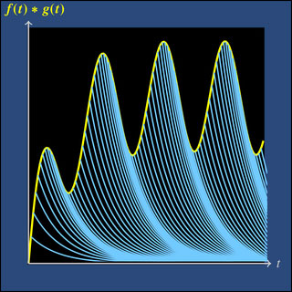
Convolution as a superposition of impulse responses. Modeled on the MIT mathlet Convolution Accumulation.

In this unit we will learn two new ways to represent certain types of functions, and these will help us solve linear time invariant (LTI) DE’s with these functions as inputs.

We start with Fourier series, which are a way to write periodic functions as sums of sinusoids. In Unit Two we learned how to solve a constant coefficient linear ODE with sinusoidal input. Now using Fourier series and the superposition principle we will be able to solve these equations with any periodic input.

Next we will study the Laplace transform. This operation transforms a given function to a new function in a different independent variable. For example, the Laplace transform of ƒ(t) = cos(3t) is F(s) = s / (s² + 9). If we think of ƒ(t) as an input signal, then the key fact is that its Laplace transform F(s) represents the same signal viewed in a different way. The Laplace transform converts a DE for the function x(t) into an algebraic equation for its Laplace transform X(s). Then, once we solve for X(s) we can recover x(t).

In the course of this unit, two important ideas will be introduced. The first is the convolution product of two functions. At first meeting this operation may seem a bit strange. Nonetheless, as we will see, it arises naturally, and the Laplace transform will allow us to work easily with it.

The second important idea is the delta function. Up to now all inputs to our systems have caused small changes in a small amount of time. An impulse is an input that causes a sudden jump in the system. For example, a sharp blow to a mass will cause its momentum to jump. The delta function is a mathematical idealization of an impulse and one which allows us to handle DE’s with these types of inputs.

« Previous | Next »

« Previous | Next »

Session Overview

We define convolution and use it in Green’s formula, which connects the response to arbitrary input q(t) with the unit impulse response.

Session Activities

Read the course notes:

Watch the lecture video clips:

Read the course notes:

Learn from the Mathlet materials:

Watch the problem solving video:

Complete the practice problems:

Check Yourself

Complete the problem set:

(Note: There is no Problem Set Part 1 for this session).

« Previous | Next »

« Previous | Next »

Advice before trying the exam:

First re-read the introduction to this unit for an overview. Next, look at the titles of the sessions and notes in the unit to remind yourself in more detail what is covered. It is also a good practice to create and solve your own practice problems.

When you have reviewed the material and think that you are ready to take the exam, write the practice exam and then check the solutions to see what you may need to review further.

« Previous | Next »

« Previous | Next »

Session Overview

We introduce general periodic functions and learn how to express them as Fourier series, which are sums of sines and cosines.

Session Activities

Read the course notes:

Check Yourself

Take the quizzes:

Session Activities

Watch the lecture video clip:

Read the course notes:

Watch the lecture video clip:

Read the course notes:

Watch the lecture video clip:

Read the course notes:

Watch the problem solving video:

Complete the practice problems:

Check Yourself

Complete the problem sets:

« Previous | Next »

« Previous | Next »

Session Overview

We introduce the Laplace transform. This is an important session which covers both the conceptual and beginning computational aspects of the topic. Fortunately, we have lots of Professor Mattuck’s videos to complement the written exposition.

Session Activities

Read the course notes:

Watch the lecture video clip:

Read the course notes:

Watch the lecture video clips:

Read the course notes:

Watch the lecture video clips:

Read the course notes:

Check Yourself

Take the quiz:

Session Activities

Read the course notes:

Watch the problem solving video:

Complete the practice problems:

Check Yourself

Complete the problem sets:

« Previous | Next »

« Previous | Next »

Session Overview

In this session we show the simple relation between the Laplace transform of a function and the Laplace transform of its derivative. We use this to help solve initial value problems for constant coefficient DE’s.

Session Activities

Read the course notes:

Watch the problem solving video:

Complete the practice problems:

Check Yourself

Complete the problem sets:

« Previous | Next »

« Previous | Next »

Session Overview

We learn how to solve constant coefficient DE’s with periodic input. The method is to use the solution for a single sinusoidal input, which we developed in Unit 2, and then superposition and the Fourier series for the input. We also discuss the relationship of Fourier series to sound waves.

Session Activities

Read the course notes:

Watch the lecture video clip:

Read the course notes:

Learn from the Mathlet materials:

Read the course notes:

Watch the lecture video clips:

Learn from the Mathlet materials:

Watch the problem solving video:

Complete the practice problems:

Check Yourself

Complete the problem sets:

« Previous | Next »

« Previous | Next »

Session Overview

In this session we will learn some tricks to help compute Fourier series, and also see in what sense a periodic function equals its Fourier series.

Session Activities

Read the course notes:

Complete the practice problem:

Watch the lecture video clip:

Read the course notes:

Watch the lecture video clip:

Read the course notes:

Learn from the Mathlet materials:

Read the course notes:

Watch the problem solving video:

Complete the practice problems:

Check Yourself

Complete the problem sets:

« Previous | Next »

« Previous | Next »

Session Overview

We learn how to compute the inverse Laplace transform. The main techniques are table lookup and partial fractions.

Session Activities

Read the course notes:

Watch the lecture video clip:

Watch the problem solving video:

Complete the practice problems:

Check Yourself

Complete the problem set:

« Previous | Next »

« Previous | Next »

Session Overview

Poles summarize the stability of a system, the rate it returns to equilibrium after its been disturbed, and the gain of the system in response to sinusoidal input. In this session we will define the poles of a system, learn their properties and how to use pole diagrams to represent them visually.

Session Activities

Read the course notes:

Learn from the Mathlet materials:

Watch the problem solving video:

Check Yourself

Complete the problem sets:

« Previous | Next »

« Previous | Next »

Session Overview

This session looks closely at discontinuous functions and introduces the notion of an impulse or delta function. The goal is to use these functions as the input to differential equations. Step functions and delta functions are not differentiable in the usual sense, but they do have what we will call generalized derivatives, which are suitable for use in DE’s.

Session Activities

Read the course notes:

Check Yourself

Take the quiz:

Session Activities

Read the course notes:

Check Yourself

Take the quizzes:

Session Activities

Watch the problem solving video:

Complete the practice problems:

Check Yourself

Complete the problem set:

(Please note: There is no Problem Set Part I for this session.)

« Previous | Next »

« Previous | Next »

Session Overview

This session ties together convolution, Laplace transform, unit impulse response and Green’s formula. They all meet in the notion of a transfer function (also known as a system function). We will define the transfer function and explore its uses in understanding systems and in combining simple systems to form more complex ones.

Session Activities

Read the course notes:

Check Yourself

Take the quizzes:

Session Activities

Read the course notes:

Watch the lecture video clip:

Read the course notes:

Check Yourself

Complete the problem sets:

« Previous | Next »

« Previous | Next »

Session Overview

In this session we study differential equations with step or delta functions as input. For physical systems, this means that we are looking at discontinuous or impulsive inputs to the system.

Session Activities

Read the course notes:

Check Yourself

Take the quiz:

Session Activities

Read the course notes:

Check Yourself

Take the quiz:

Session Activities

Read the course notes:

Check Yourself

Take the quiz:

Session Activities

Read the course notes:

Watch the problem solving video:

Complete the practice problems:

Check Yourself

Complete the problem sets:

« Previous | Next »

Course Info

Learning Resource Types
Lecture Videos
Recitation Videos
Exams with Solutions
Simulations
Lecture Notes
Problem Sets with Solutions