The Lab Experiments are linked below. Please note that Lab Experiment IX was skipped (as shown in the calendar) and Lab Experiment XV is not available to OCW users.
GFD0: Rotation stiffens fluids
GFDI: Cloud formation on adiabatic expansion
GFDII: Convection
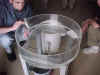
GFDIII: Radial inflow
GFDIV: Parabolic table
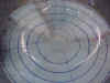
GFDV: Inertial circles
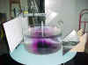
GFDVI: Perrot’s bathtub experiment
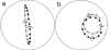
GFDVII: Taylor columns
GFDVIII: Thermal wind and Hadley circulation
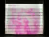
GFDIX: Slope of a frontal surface
GFDX: Ekman layers
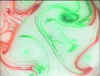
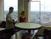
GFDXI: Atmospheric general circulation
GFDXII: Ekman pumping and suction
GFDXIII: Ocean gyres
GFDXIV: Thermohaline circulation
GFD0: Rotation stiffens fluids
GFDI: Cloud formation on adiabatic expansion 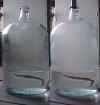
GFDVI: Perrot’s bathtub experiment
GFDVIII: Thermal wind and Hadley circulation
GFDIX: Slope of a frontal surface
GFDXI: Atmospheric general circulation