
L21: Parallel Processing
- Processor Performance
- 5-Stage Pipelined Processors
- Improving 5-Stage Pipeline Performance
- Limits to Pipeline Depth
- Improving 5-Stage Pipeline Performance
- Instruction-level Parallelism (ILP)
- Wider or Superscalar Pipelines
- A Modern Out-of-Order Superscalar Processor
- Limits to Single-Processor Performance
- Data-Level Parallelism
- Vector Code Example
- Data-Dependent Vector Operations
- Vector Processing Implementations
- Multicore Processors
- Amdahl’s Law
- Amdahl’s Law and Parallelism
- Thread-Level Parallelism
- Multicore Caches
- What Are the Possible Outcomes
- Uniprocessor Outcome
- Sequential Consistency
- Alternatives to Sequential Consistency?
- Fix: “Snoopy” Cache Coherence Protocol
- Example: MESI Cache Coherence Protocol
- The Cache Has Two Customers!
- MESI Activity Diagram
- Cache Coherence in Action
- Parallel Processing Summary
Content of the following slides is described in the surrounding text.
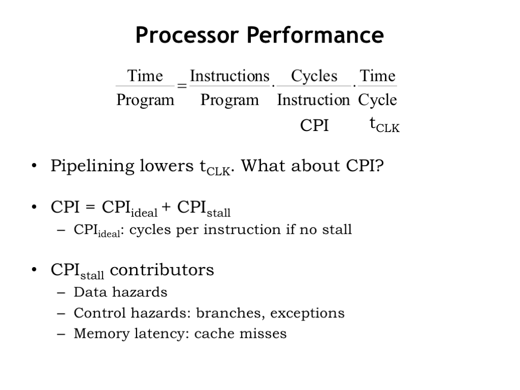
The modern world has an insatiable appetite for computation, so system architects are always thinking about ways to make programs run faster. The running time of a program is the product of three terms:
The number of instructions in the program, multiplied by the average number of processor cycles required to execute each instruction (CPI), multiplied by the time required for each processor cycle (\(t_{\textrm{CLK}}\)).
To decrease the running time we need to decrease one or more of these terms. The number of instructions per program is determined by the ISA and by the compiler that produced the sequence of assembly language instructions to be executed. Both are fair game, but for this discussion, let’s work on reducing the other two terms.
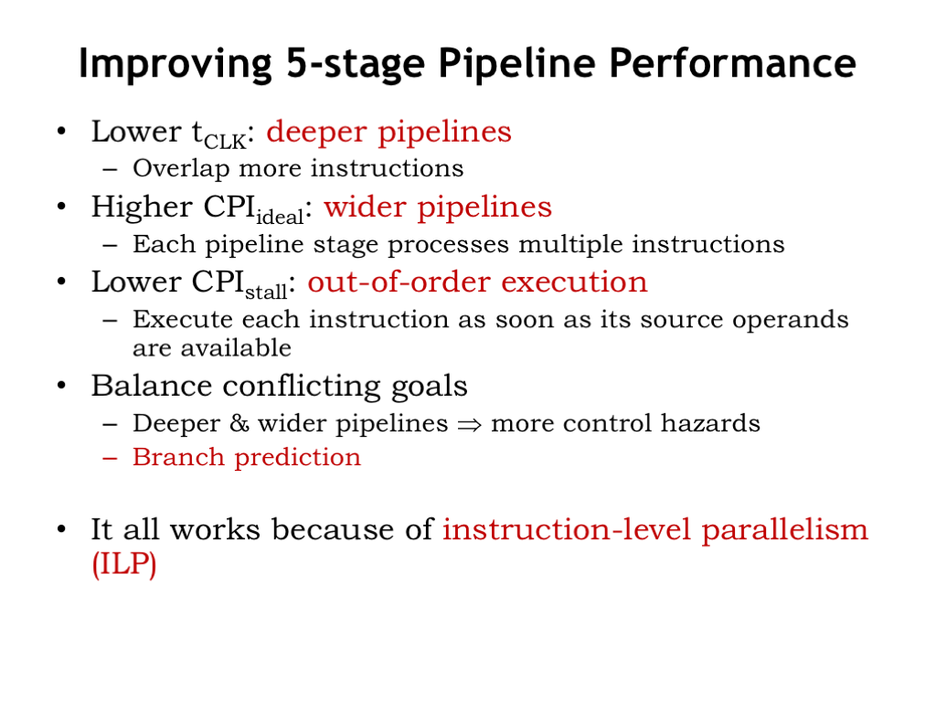
As we’ve seen, pipelining reduces \(t_{\textrm{CLK}}\) by dividing instruction execution into a sequence of steps, each of which can complete its task in a shorter \(t_{\textrm{CLK}}\). What about reducing CPI?
In our 5-stage pipelined implementation of the Beta, we designed the hardware to complete the execution of one instruction every clock cycle, so CPI_ideal is 1. But sometimes the hardware has to introduce “NOP bubbles” into the pipeline to delay execution of a pipeline stage if the required operation couldn’t (yet) be completed. This happens on taken branch instructions, when attempting to immediately use a value loaded from memory by the LD instruction, and when waiting for a cache miss to be satisfied from main memory. CPI_stall accounts for the cycles lost to the NOPs introduced into the pipeline. Its value depends on the frequency of taken branches and immediate use of LD results. Typically it’s some fraction of a cycle. For example, if a 6-instruction loop with a LD takes 8 cycles to complete, CPI_stall for the loop would be 2/6, i.e., 2 extra cycles for every 6 instructions.
Our classic 5-stage pipeline is an effective compromise that allows for a substantial reduction of \(t_{\textrm{CLK}}\) while keeping CPI_stall to a reasonably modest value.
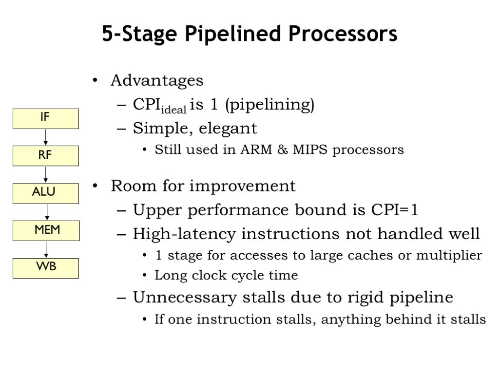
There is room for improvement. Since each stage is working on one instruction at a time, CPI_ideal is 1.
Slow operations — e.g., completing a multiply in the ALU stage, or accessing a large cache in the IF or MEM stages — force \(t_{\textrm{CLK}}\) to be large to accommodate all the work that has to be done in one cycle.
The order of the instructions in the pipeline is fixed. If, say, a LD instruction is delayed in the MEM stage because of a cache miss, all the instructions in earlier stages are also delayed even though their execution may not depend on the value produced by the LD. The order of instructions in the pipeline always reflects the order in which they were fetched by the IF stage.
Let’s look into what it would take to relax these constraints and hopefully improve program runtimes.
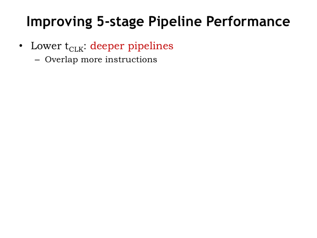
Increasing the number of pipeline stages should allow us to decrease the clock cycle time. We’d add stages to break up performance bottlenecks, e.g., adding additional pipeline stages (MEM1 and MEM2) to allow a longer time for memory operations to complete. This comes at cost to CPI_stall since each additional MEM stage means that more NOP bubbles have to be introduced when there’s a LD data hazard. Deeper pipelines mean that the processor will be executing more instructions in parallel.
Let’s interrupt enumerating our performance shopping list to think about limits to pipeline depth.
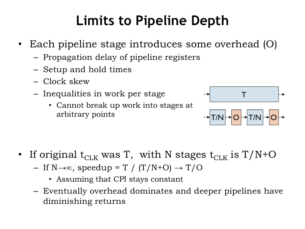
Each additional pipeline stage includes some additional overhead costs to the time budget. We have to account for the propagation, setup, and hold times for the pipeline registers. And we usually have to allow a bit of extra time to account for clock skew, i.e., the difference in arrival time of the clock edge at each register. And, finally, since we can’t always divide the work exactly evenly between the pipeline stages, there will be some wasted time in the stages that have less work. We’ll capture all of these effects as an additional per-stage time overhead of O.
If the original clock period was T, then with N pipeline stages, the clock period will be T/N + O.
At the limit, as N becomes large, the speedup approaches T/O. In other words, the overhead starts to dominate as the time spent on work in each stage becomes smaller and smaller. At some point adding additional pipeline stages has almost no impact on the clock period.
As a data point, the Intel Core-2 x86 chips (nicknamed “Nehalem”) have a 14-stage execution pipeline.
Okay, back to our performance shopping list…
There may be times we can arrange to execute two or more instructions in parallel, assuming that their executions are independent from each other. This would increase CPI_ideal at the cost of increasing the complexity of each pipeline stage to deal with concurrent execution of multiple instructions.
If there’s an instruction stalled in the pipeline by a data hazard, there may be following instructions whose execution could still proceed. Allowing instructions to pass each other in the pipeline is called out-of-order execution. We’d have to be careful to ensure that changing the execution order didn’t affect the values produced by the program.
More pipeline stages and wider pipeline stages increase the amount of work that has to be discarded on control hazards, potentially increasing CPI_stall. So it’s important to minimize the number of control hazards by predicting the results of a branch (i.e., taken or not taken) so that we increase the chances that the instructions in the pipeline are the ones we’ll want to execute.
Our ability to exploit wider pipelines and out-of-order execution depends on finding instructions that can be executed in parallel or in different orders. Collectively these properties are called “instruction-level parallelism” (ILP).
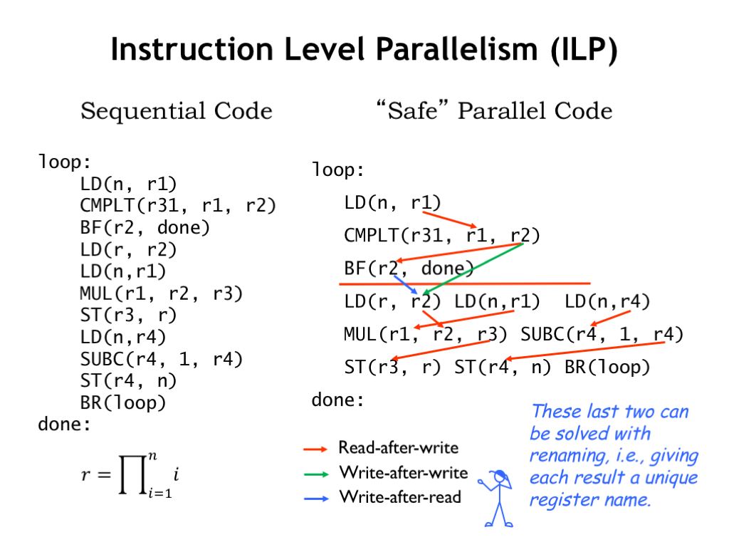
Here’s an example that will let us explore the amount of ILP that might be available. On the left is an unoptimized loop that computes the product of the first N integers. On the right, we’ve rewritten the code, placing instructions that could be executed concurrently on the same line.
First notice the red line following the BF instruction. Instructions below the line should only be executed if the BF is *not* taken. That doesn’t mean we couldn’t start executing them before the results of the branch are known, but if we executed them before the branch, we would have to be prepared to throw away their results if the branch was taken.
The possible execution order is constrained by the read-after-write (RAW) dependencies shown by the red arrows. We recognize these as the potential data hazards that occur when an operand value for one instruction depends on the result of an earlier instruction. In our 5-stage pipeline, we were able to resolve many of these hazards by bypassing values from the ALU, MEM, and WB stages back to the RF stage where operand values are determined.
Of course, bypassing will only work when the instruction has been executed so its result is available for bypassing! So in this case, the arrows are showing us the constraints on execution order that guarantee bypassing will be possible.
There are other constraints on execution order. The green arrow identifies a write-after-write (WAW) constraint between two instructions with the same destination register. In order to ensure the correct value is in R2 at the end of the loop, the LD(r,R2) instruction has to store its result into the register file after the result of the CMPLT instruction is stored into the register file.
Similarly, the blue arrow shows a write-after-read (WAR) constraint that ensures that the correct values are used when accessing a register. In this case, LD(r,R2) must store into R2 after the Ra operand for the BF has been read from R2.
As it turns out, WAW and WAR constraints can be eliminated if we give each instruction result a unique register name. This can actually be done relatively easily by the hardware by using a generous supply of temporary registers, but we won’t go into the details of renaming here. The use of temporary registers also makes it easy to discard results of instructions executed before we know the outcomes of branches.
In this example, we discovered that the potential concurrency was actually pretty good for the instructions following the BF.
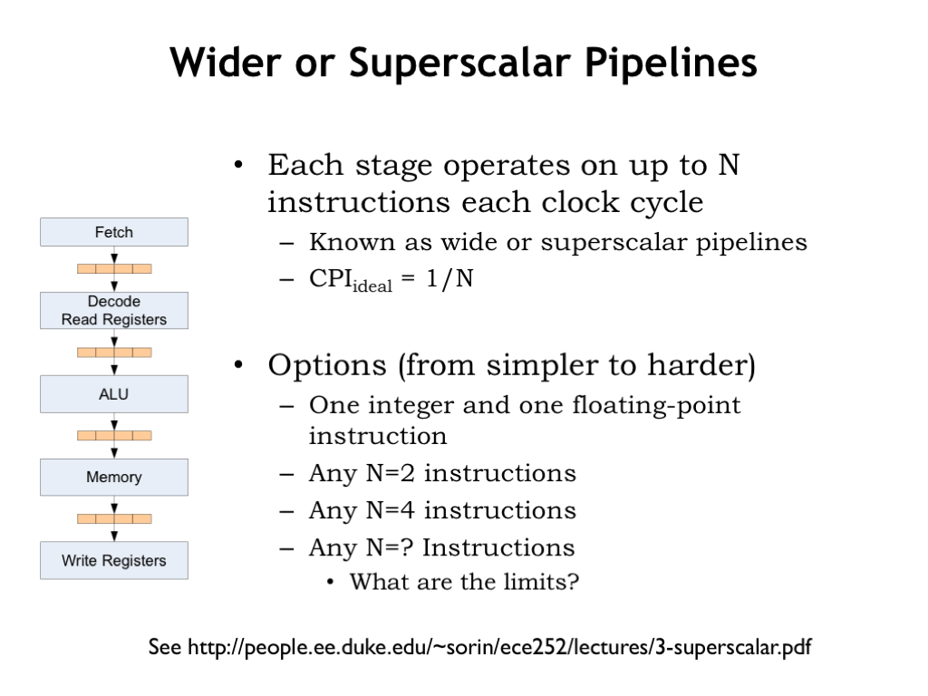
To take advantage of this potential concurrency, we’ll need to modify the pipeline to execute some number N of instructions in parallel. If we can sustain that rate of execution, CPI_ideal would then be 1/N since we’d complete the execution of N instructions in each clock cycle as they exited the final pipeline stage.
So what value should we choose for N? Instructions that are executed by different ALU hardware are easy to execute in parallel, e.g., ADDs and SHIFTs, or integer and floating-point operations. Of course, if we provided multiple adders, we could execute multiple integer arithmetic instructions concurrently. Having separate hardware for address arithmetic (called LD/ST units) would support concurrent execution of LD/ST instructions and integer arithmetic instructions.
This set of lecture slides from Duke gives a nice overview of techniques used in each pipeline stage to support concurrent execution.
Basically by increasing the number of functional units in the ALU and the number of memory ports on the register file and main memory, we would have what it takes to support concurrent execution of multiple instructions. So, what’s the right tradeoff between increased circuit costs and increased concurrency?
As a data point, the Intel Nehalem core can complete up to 4 micro-operations per cycle, where each micro-operation corresponds to one of our simple RISC instructions.
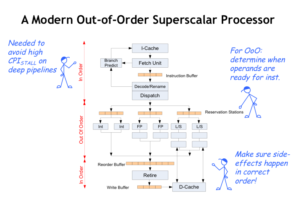
Here’s a simplified diagram of a modern out-of-order superscalar processor.
Instruction fetch and decode handles, say, 4 instructions at a time. The ability to sustain this execution rate depends heavily on the ability to predict the outcome of branch instructions, ensuring that the wide pipeline will be mostly filled with instructions we actually want to execute. Good branch prediction requires the use of the history from previous branches and there’s been a lot of cleverness devoted to getting good predictions from the least amount of hardware! If you’re interested in the details, search for “branch predictor” on Wikipedia.
The register renaming happens during instruction decode, after which the instructions are ready to be dispatched to the functional units.
If an instruction needs the result of an earlier instruction as an operand, the dispatcher has identified which functional unit will be producing the result. The instruction waits in a queue until the indicated functional unit produces the result and when all the operand values are known, the instruction is finally taken from the queue and executed. Since the instructions are executed by different functional units as soon as their operands are available, the order of execution may not be the same as in the original program.
After execution, the functional units broadcast their results so that waiting instructions know when to proceed. The results are also collected in a large reorder buffer so that they can be retired (i.e., write their results in the register file) in the correct order.
Whew! There’s a lot of circuitry involved in keeping the functional units fed with instructions, knowing when instructions have all their operands, and organizing the execution results into the correct order. So how much speed up should we expect from all this machinery? The effective CPI is very program-specific, depending as it does on cache hit rates, successful branch prediction, available ILP, and so on. Given the architecture described here the best speed up we could hope for is a factor of 4. Googling around, it seems that the reality is an average speed-up of 2, maybe slightly less, over what would be achieved by an in-order, single-issue processor.
What can we expect for future performance improvements in out-of-order, superscalar pipelines?
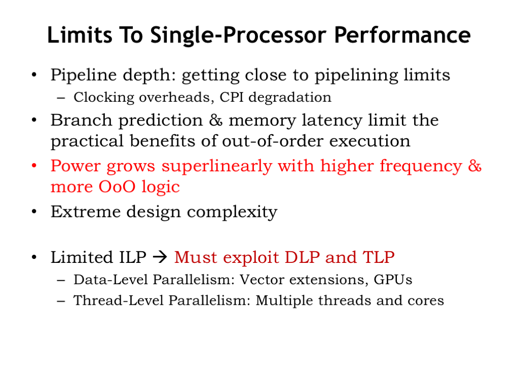
Increases in pipeline depth can cause CPI_stall and timing overheads to rise. At the current pipeline depths the increase in CPI_stall is larger than the gains from decreased \(t_{\textrm{CLK}}\) and so further increases in depth are unlikely.
A similar tradeoff exists between using more out-of-order execution to increase ILP and the increase in CPI_stall caused by the impact of mis-predicted branches and the inability to run main memories any faster.
Power consumption increases more quickly than the performance gains from lower \(t_{\textrm{CLK}}\) and additional out-of-order execution logic.
The additional complexity required to enable further improvements in branch prediction and concurrent execution seems very daunting.
All of these factors suggest that is unlikely that we’ll see substantial future improvements in the performance of out-of-order superscalar pipelined processors.
So system architects have turned their attention to exploiting data-level parallelism (DLP) and thread-level parallelism (TLP). These are our next two topics.
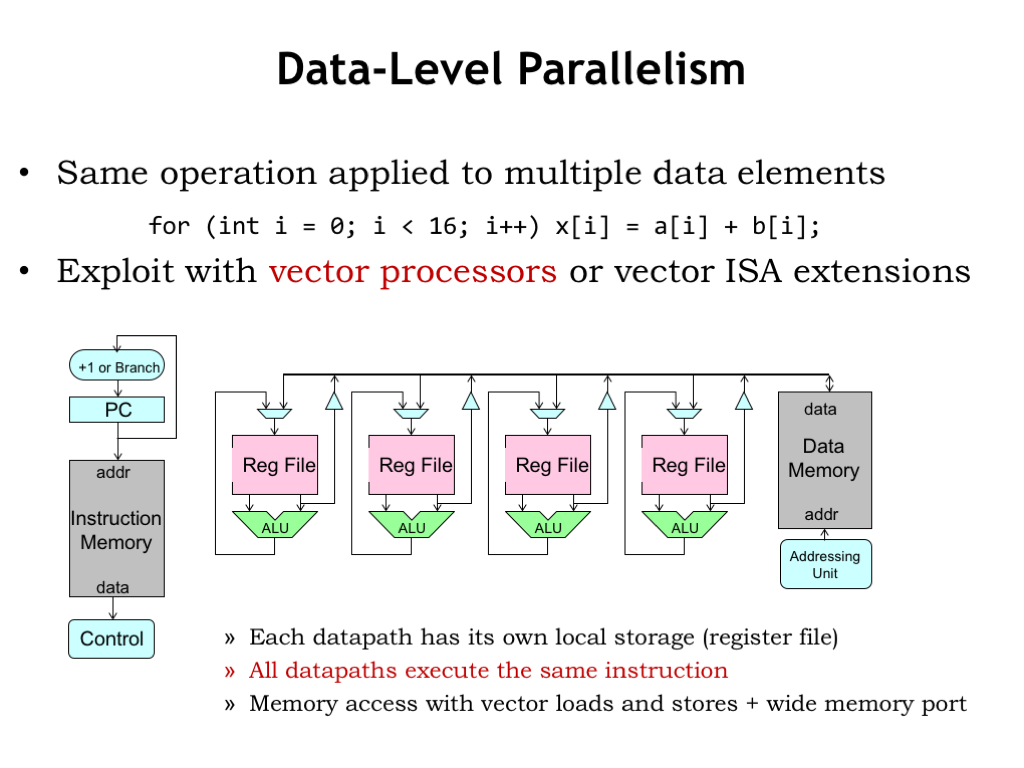
For some applications, data naturally comes in vector or matrix form. For example, a vector of digitized samples representing an audio waveform over time, or an matrix of pixel colors in a 2D image from a camera. When processing that data, it’s common to perform the same sequence of operations on each data element. The example code shown here is computing a vector sum, where each component of one vector is added to the corresponding component of another vector.
By replicating the datapath portion of our CPU, we can design special-purpose vector processors capable of performing the same operation on many data elements in parallel. Here we see that the register file and ALU have been replicated and the control signals from decoding the current instruction are shared by all the datapaths. Data is fetched from memory in big blocks (very much like fetching a cache line) and the specified register in each datapath is loaded with one of the words from the block. Similarly each datapath can contribute a word to be stored as a contiguous block in main memory. In such machines, the width of the data buses to and from main memory is many words wide, so a single memory access provides data for all the datapaths in parallel.
Executing a single instruction on a machine with N datapaths is equivalent to executing N instructions on a conventional machine with a single datapath. The result achieves a lot of parallelism without the complexities of out-of-order superscalar execution.
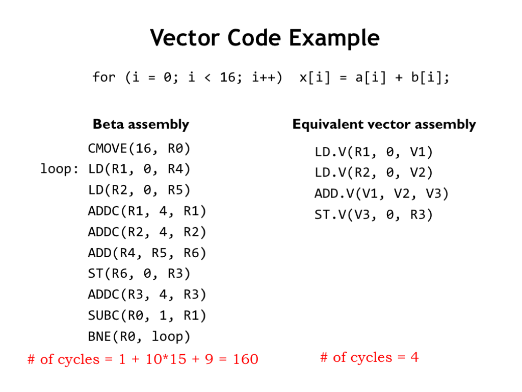
Suppose we had a vector processor with 16 datapaths. Let’s compare its performance on a vector-sum operation to that of a conventional pipelined Beta processor.
Here’s the Beta code, carefully organized to avoid any data hazards during execution. There are 9 instructions in the loop, taking 10 cycles to execute if we count the NOP introduced into the pipeline when the BNE at the end of the loop is taken. It takes 160 cycles to sum all 16 elements assuming no additional cycles are required due to cache misses.
And here’s the corresponding code for a vector processor where we’ve assumed constant-sized 16-element vectors. Note that “V” registers refer to a particular location in the register file associated with each datapath, while the “R” registers are the conventional Beta registers used for address computations, etc. It would only take 4 cycles for the vector processor to complete the desired operations, a speed-up of 40.
This example shows the best-possible speed-up. The key to a good speed-up is our ability to “vectorize” the code and take advantage of all the datapaths operating in parallel. This isn’t possible for every application, but for tasks like audio or video encoding and decoding, and all sorts of digital signal processing, vectorization is very doable. Memory operations enjoy a similar performance improvement since the access overhead is amortized over large blocks of data.
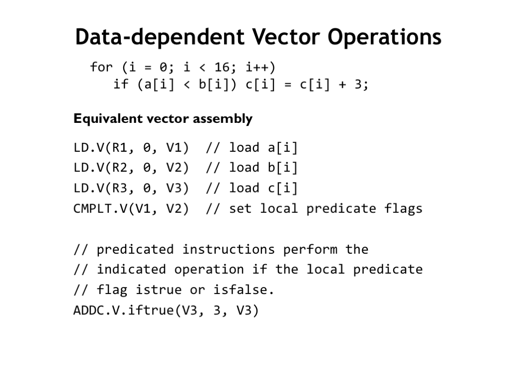
You might wonder if it’s possible to efficiently perform data-dependent operations on a vector processor. Data-dependent operations appear as conditional statements on conventional machines, where the body of the statement is executed if the condition is true. If testing and branching is under the control of the single instruction execution engine, how can we take advantage of the parallel datapaths?
The trick is provide each datapath with a local predicate flag. Use a vectorized compare instruction (CMPLT.V) to perform the a[i] < b[i] comparisons in parallel and remember the result locally in each datapath’s predicate flag. Then extend the vector ISA to include “predicated instructions” which check the local predicate to see if they should execute or do nothing. In this example, ADDC.V.iftrue only performs the ADDC on the local data if the local predicate flag is true.
Instruction predication is also used in many non-vector architectures to avoid the execution-time penalties associated with mis-predicted conditional branches. They are particularly useful for simple arithmetic and boolean operations (i.e., very short instruction sequences) that should be executed only if a condition is met. The x86 ISA includes a conditional move instruction, and in the 32-bit ARM ISA almost all instructions can be conditionally executed.
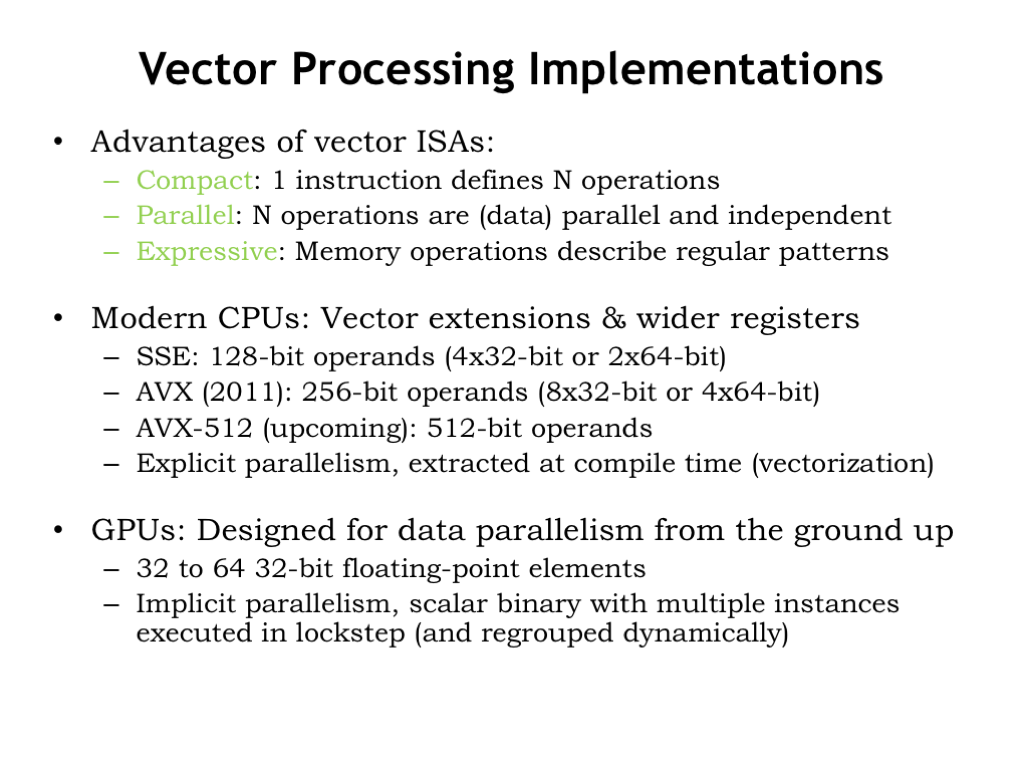
The power of vector processors comes from having 1 instruction initiate N parallel operations on N pairs of operands.
Most modern CPUs incorporate vector extensions that operate in parallel on 8-, 16-, 32- or 64-bit operands organized as blocks of 128-, 256-, or 512-bit data. Often all that’s needed is some simple additional logic on an ALU designed to process full-width operands. The parallelism is baked into the vector program, not discovered on-the-fly by the instruction dispatch and execution machinery. Writing the specialized vector programs is a worthwhile investment for certain library functions which see a lot use in processing today’s information streams with their heavy use of images, and A/V material.
Perhaps the best example of architectures with many datapaths operating in parallel are the graphics processing units (GPUs) found in almost all computer graphics systems. GPU datapaths are typically specialized for 32- and 64-bit floating point operations found in the algorithms needed to display in real-time a 3D scene represented as billions of triangular patches as a 2D image on the computer screen. Coordinate transformation, pixel shading and antialiasing, texture mapping, etc., are examples of “embarrassingly parallel” computations where the parallelism comes from having to perform the same computation independently on millions of different data objects. Similar problems can be found in the fields of bioinformatics, big data processing, neural net emulation used in deep machine learning, and so on. Increasingly, GPUs are used in many interesting scientific and engineering calculations and not just as graphics engines.
Data-level parallelism provides significant performance improvements in a variety of useful situations. So current and future ISAs will almost certainly include support for vector operations.

In discussing out-of-order superscalar pipelined CPUs we commented that the costs grow very quickly relative the to performance gains, leading to the cost-performance curve shown here. If we move down the curve, we can arrive at more efficient architectures that give, say, 1/2 the performance at a 1/4 of the cost.
When our applications involve independent computations that can be performed in a parallel, it may be that we would be able to use two cores to provide the same performance as the original expensive core, but a fraction of the cost. If the available parallelism allows us to use additional cores, we’ll see a linear relationship between increased performance vs. increased cost. The key, of course, is that desired computations can be divided into multiple tasks that can run independently, with little or no need for communication or coordination between the tasks.
What is the optimal tradeoff between core cost and the number of cores? If our computation is arbitrarily divisible without incurring additional overhead, then we would continue to move down the curve until we found the cost-performance point that gave us the desired performance at the least cost. In reality, dividing the computation across many cores does involve some overhead, e.g., distributing the data and code, then collecting and aggregating the results, so the optimal tradeoff is harder to find. Still, the idea of using a larger number of smaller, more efficient cores seems attractive.
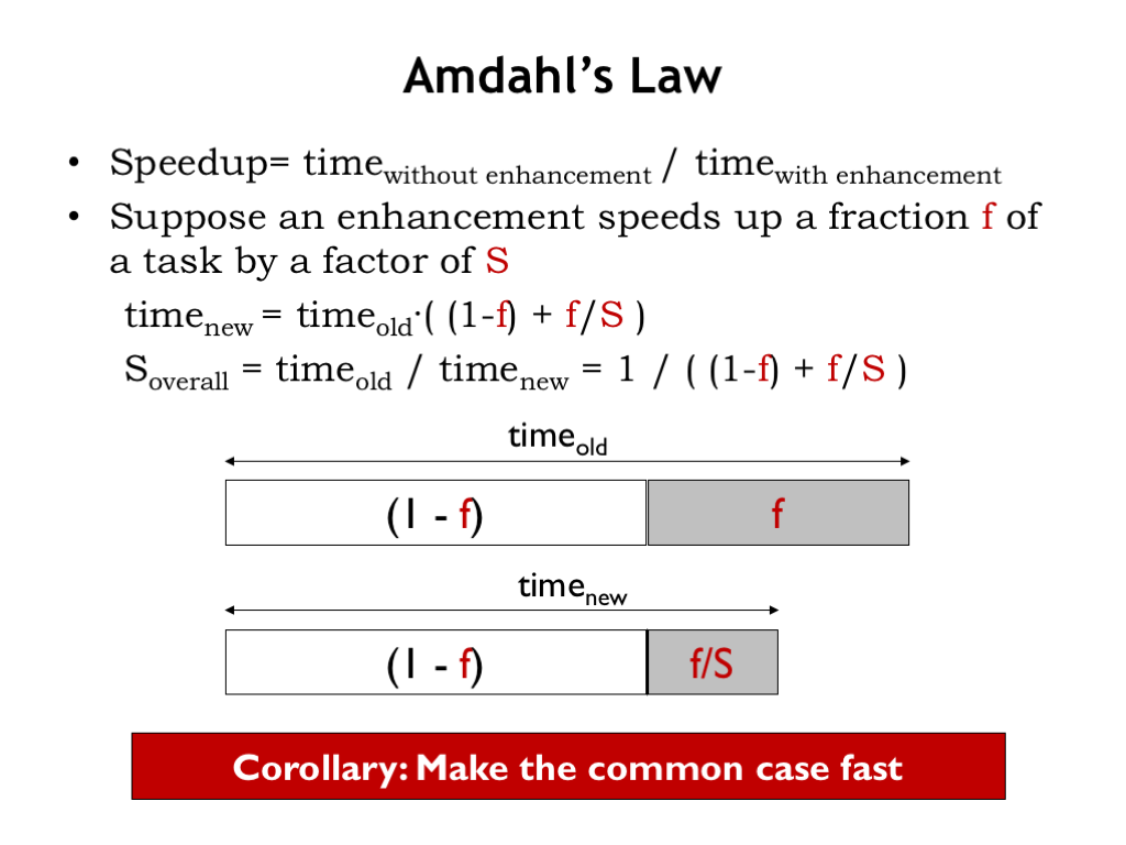
Many applications have some computations that can be performed in parallel, but also have computations that won’t benefit from parallelism. To understand the speedup we might expect from exploiting parallelism, it’s useful to perform the calculation proposed by computer scientist Gene Amdahl in 1967, now known as Amdahl’s Law.
Suppose we’re considering an enhancement that speeds up some fraction F of the task at hand by a factor of S. As shown in the figure, the gray portion of the task now takes F/S of the time that it used to require.
Some simple arithmetic lets us calculate the overall speedup we get from using the enhancement. One conclusion we can draw is that we’ll benefit the most from enhancements that affect a large portion of the required computations, i.e., we want to make F as large a possible.
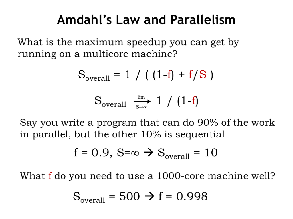
What’s the best speedup we can hope for if we have many cores that can be used to speed up the parallel part of the task? Here’s the speedup formula based on F and S, where in this case F is the parallel fraction of the task. If we assume that the parallel fraction of the task can be speed up arbitrarily by using more and more cores, we see that the best possible overall speed up is 1/(1-F).
For example, you write a program that can do 90% of its work in parallel, but the other 10% must be done sequentially. The best overall speedup that can be achieved is a factor of 10, no matter how many cores you have at your disposal.
Turning the question around, suppose you have a 1000-core machine which you hope to be able to use to achieve a speedup of 500 on your target application. You would need to be able parallelize 99.8% of the computation in order to reach your goal! Clearly multicore machines are most useful when the target task has lots of natural parallelism.
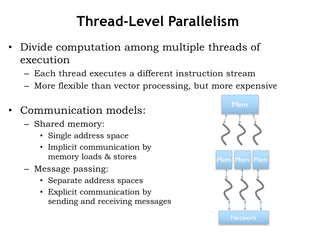
Using multiple independent cores to execute a parallel task is called thread-level parallelism (TLP), where each core executes a separate computation “thread”. The threads are independent programs, so the execution model is potentially more flexible than the lock-step execution provided by vector machines.
When there are a small number of threads, you often see the cores sharing a common main memory, allowing the threads to communicate and synchronize by sharing a common address space. We’ll discuss this further in the next section. This is the approach used in current multicore processors, which have between 2 and 12 cores.
Shared memory becomes a real bottleneck when there 10’s or 100’s of cores, since collectively they quickly overwhelm the available memory bandwidth. In these architectures, threads communicate using a communication network to pass messages back and forth. We discussed possible network topologies in an earlier lecture. A cost-effective on-chip approach is to use a nearest-neighbor mesh network, which supports many parallel point-to-point communications, while still allowing multi-hop communication between any two cores. Message passing is also used in computing clusters, where many ordinary CPUs collaborate on large tasks. There’s a standardized message passing interface (MPI) and specialized, very high throughput, low latency message-passing communication networks (e.g., Infiniband) that make it easy to build high-performance computing clusters.
In the next couple of sections we’ll look more closely at some of the issues involved in building shared-memory multicore processors.
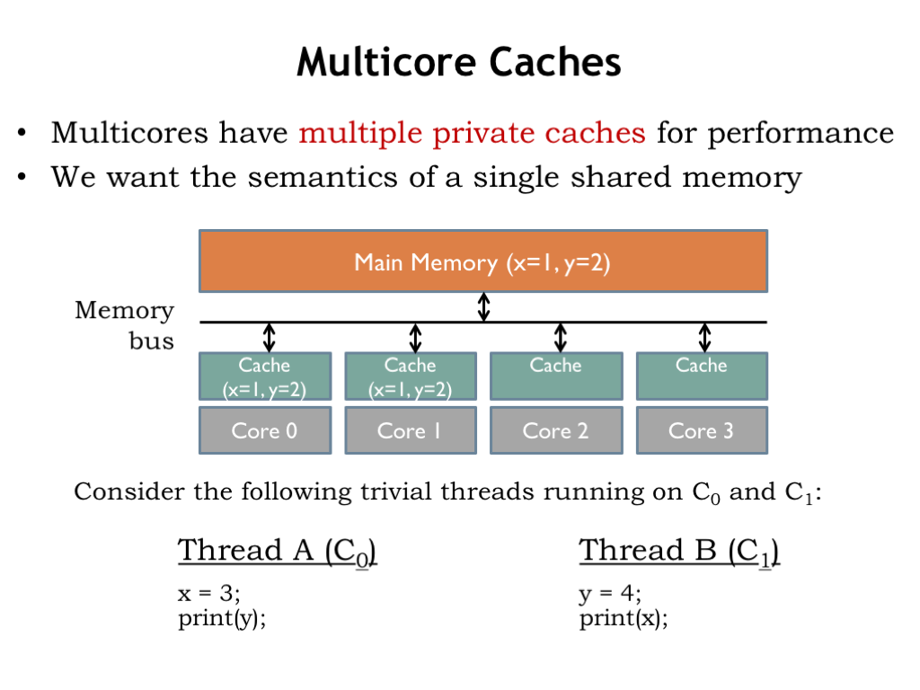
A conceptual schematic for a multicore processor is shown below. To reduce the average memory access time, each of the four cores has its own cache, which will satisfy most memory requests. If there’s a cache miss, a request is sent to the shared main memory. With a modest number of cores and a good cache hit ratio, the number of memory requests that must access main memory during normal operation should be pretty small. To keep the number of memory accesses to a minimum, the caches implement a write-back strategy, where ST instructions update the cache, but main memory is only updated when a dirty cache line is replaced.
Our goal is that each core should share the contents of main memory, i.e., changes made by one core should visible to all the other cores. In the example shown here, core 0 is running Thread A and core 1 is running Thread B. Both threads reference two shared memory locations holding the values for the variables X and Y.
The current values of X and Y are 1 and 2, respectively. Those values are held in main memory as well as being cached by each core.
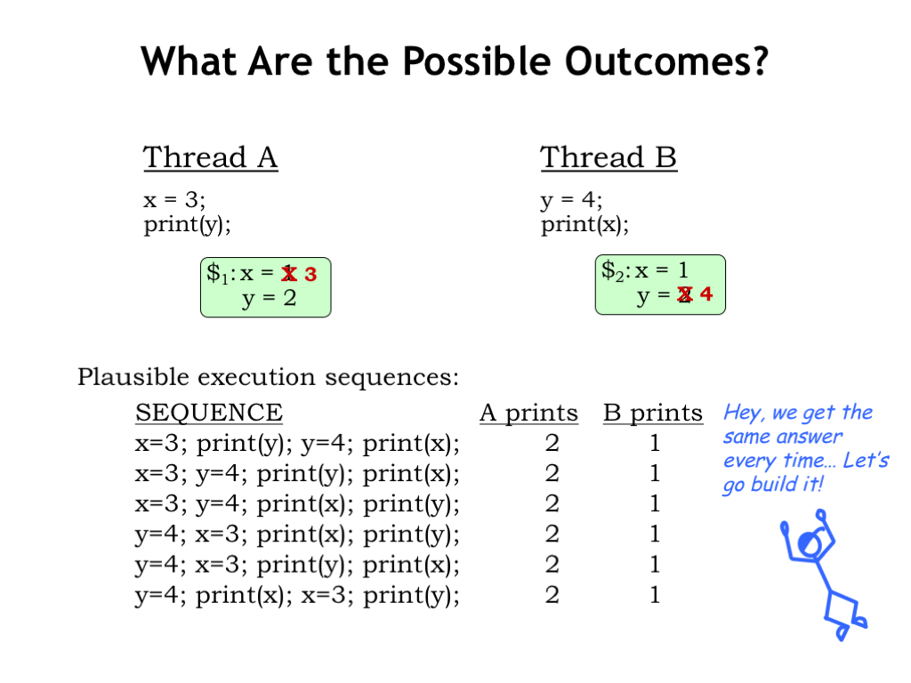
What happens when the threads are executed? Each thread executes independently, updating its cache during stores to X and Y. For any possible execution order, either concurrent or sequential, the result is the same: Thread A prints “2”, Thread B prints “1”. Hardware engineers would point to the consistent outcomes and declare victory!
But closer examination of the final system state reveals some problems. After execution is complete, the two cores disagree on the values of X and Y. Threads running on core 0 will see X=3 and Y=2. Threads running on core 1 will see X=1 and Y=4. Because of the caches, the system isn’t behaving as if there’s a single shared memory. On the other hand, we can’t eliminate the caches since that would cause the average memory access time to skyrocket, ruining any hoped-for performance improvement from using multiple cores.
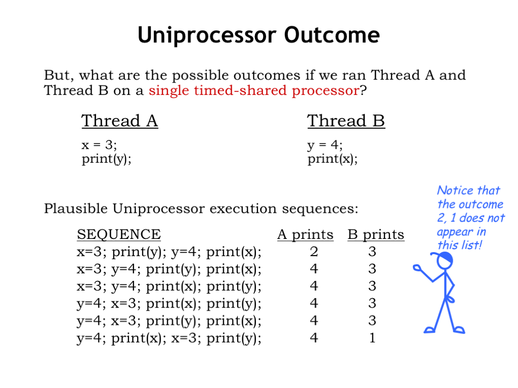
What outcome should we expect? One plausible standard of correctness is the outcome when the threads are run a single timeshared core. The argument would be that a multicore implementation should produce the same outcome but more quickly, with parallel execution replacing timesharing.
The table shows the possible results of the timesharing experiment, where the outcome depends on the order in which the statements are executed. Programmers will understand that there is more than one possible outcome and know that they would have to impose additional constraints on execution order, say, using semaphores, if they wanted a specific outcome.
Notice that the multicore outcome of 2,1 doesn’t appear anywhere on the list of possible outcomes from sequential timeshared execution.
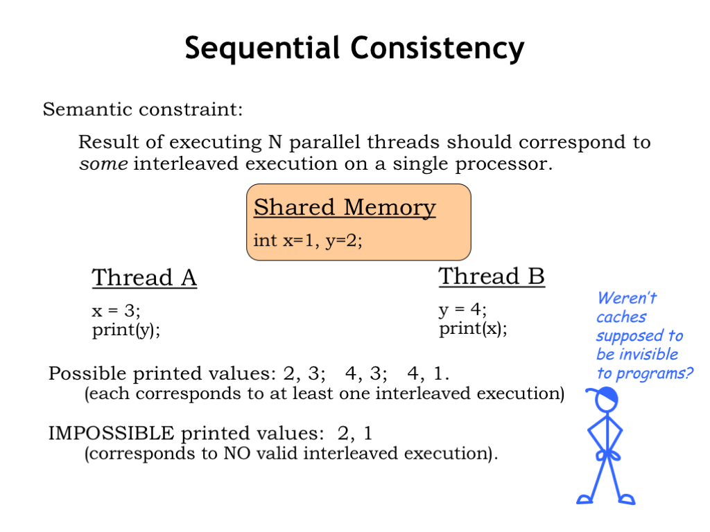
The notion that executing N threads in parallel should correspond to some interleaved execution of those threads on a single core is called “sequential consistency”. If multicore systems implement sequential consistency, then programmers can think of the systems as providing hardware-accelerated timesharing.
So, our simple multicore system fails on two accounts. First, it doesn’t correctly implement a shared memory since, as we’ve seen, it’s possible for the two cores to disagree about the current value of a shared variable. Second, as a consequence of the first problem, the system doesn’t implement sequential consistency.
Clearly, we’ll need to figure out a fix!
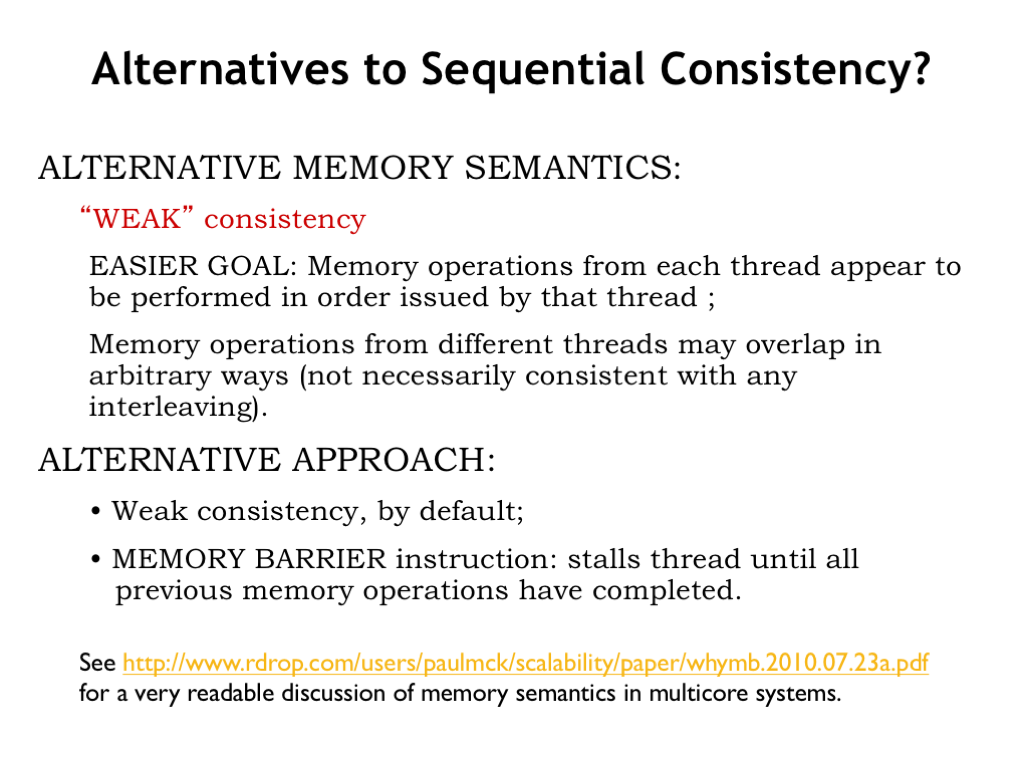
One possible fix is to give up on sequential consistency. An alternative memory semantics is “weak consistency”, which only requires that the memory operations from each thread appear to be performed in the order issued by that thread. In other words in a weakly consistent system, if a particular thread writes to X and then writes to Y, the possible outcomes from reads of X and Y by any thread would be one of
(unchanged X, unchanged Y), or (changed X, unchanged Y), or (changed X, changed Y).
But no thread would see changed Y but unchanged X.
In a weakly consistent system, memory operations from other threads may overlap in arbitrary ways (not necessarily consistent with any sequential interleaving).
Note that our multicore cache system doesn’t itself guarantee even weak consistency. A thread that executes “write X; write Y” will update its local cache, but later cache replacements may cause the updated Y value to be written to main memory before the updated X value. To implement weak consistency, the thread should be modified to “write X; communicate changes to all other processors; write Y”. In the next section, we’ll discuss how to modify the caches to perform the required communication automatically.
Out-of-order cores have an extra complication since there’s no guarantee that successive ST instructions will complete in the order they appeared in the program. These architectures provide a BARRIER instruction that guarantees that memory operations before the BARRIER are completed before memory operation executed after the BARRIER.
There are many types of memory consistency — each commercially-available multicore system has its own particular guarantees about what happens when. So the prudent programmer needs to read the ISA manual carefully to ensure that her program will do what she wants. See the referenced PDF file for a very readable discussion about memory semantics in multicore systems.
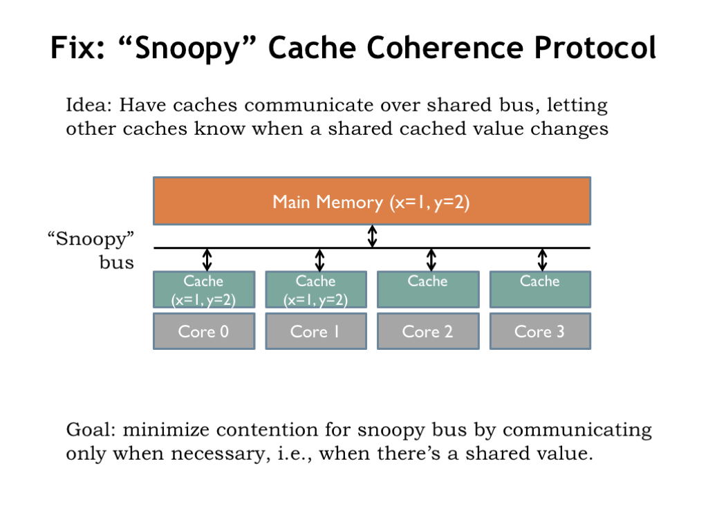
The problem with our simple multicore system is that there is no communication when the value of a shared variable is changed. The fix is to provide the necessary communications over a shared bus that’s watched by all the caches. A cache can then “snoop” on what’s happening in other caches and then update its local state to be consistent. The required communications protocol is called a “cache coherence protocol”.
In designing the protocol, we’d like to incur the communications overhead only when there’s actual sharing in progress, i.e., when multiple caches have local copies of a shared variable.
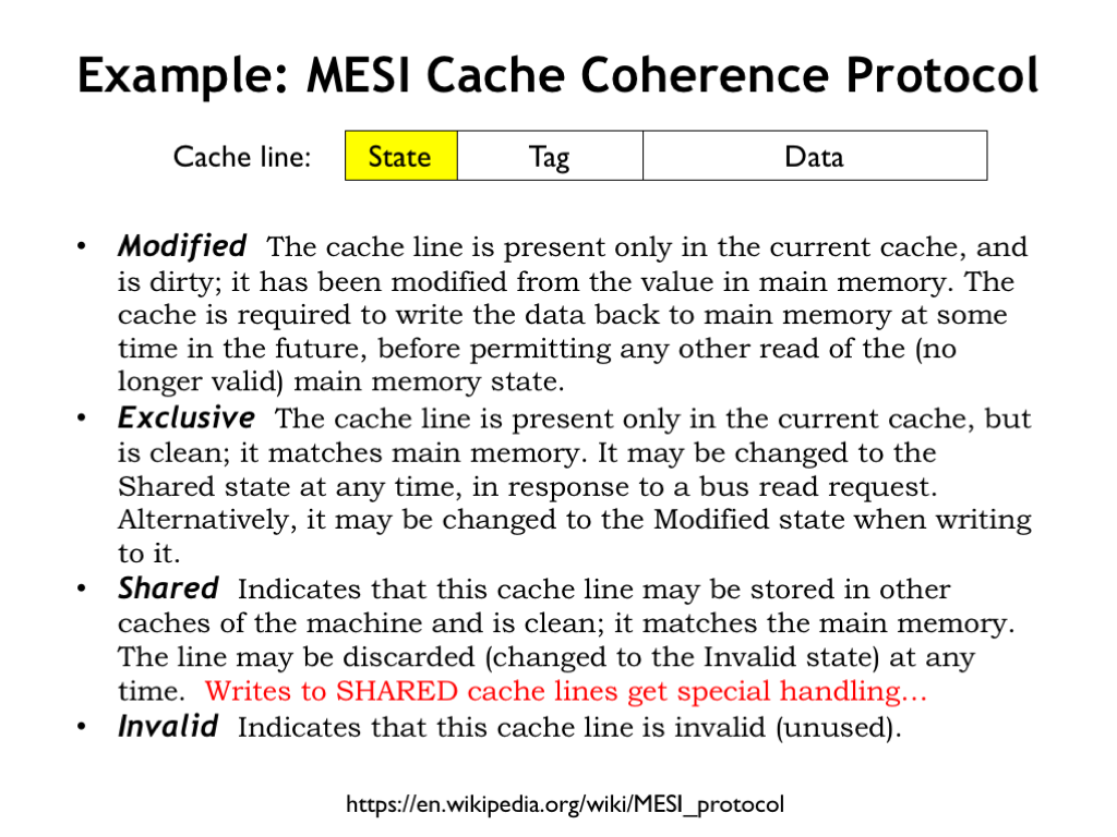
To implement a cache coherence protocol, we’ll change the state maintained for each cache line.
The initial state for all cache lines is INVALID indicating that the tag and data fields do not contain up-to-date information. This corresponds to setting the valid bit to 0 in our original cache implementation.
When the cache line state is EXCLUSIVE, this cache has the only copy of those memory locations and indicates that the local data is the same as that in main memory. This corresponds to setting the valid bit to 1 in our original cache implementation.
If the cache line state is MODIFIED, that means the cache line data is the sole valid copy of the data. This corresponds to setting both the dirty and valid bits to 1 in our original cache implementation.
To deal with sharing issues, there’s a fourth state called SHARED that indicates when other caches may also have a copy of the same unmodified memory data.
When filling a cache from main memory, other caches can snoop on the read access and participate if fulfilling the read request.
If no other cache has the requested data, the data is fetched from main memory and the requesting cache sets the state of that cache line to EXCLUSIVE.
If some other cache has the requested in line in the EXCLUSIVE or SHARED state, it supplies the data and asserts the SHARED signal on the snoopy bus to indicate that more than one cache now has a copy of the data. All caches will mark the state of the cache line as SHARED.
If another cache has a MODIFIED copy of the cache line, it supplies the changed data, providing the correct values for the requesting cache as well as updating the values in main memory. Again the SHARED signal is asserted and both the reading and responding cache will set the state for that cache line to SHARED.
So, at the end of the read request, if there are multiple copies of the cache line, they will all be in the SHARED state. If there’s only one copy of the cache line it will be in the EXCLUSIVE state.
Writing to a cache line is when the sharing magic happens. If there’s a cache miss, the first cache performs a cache line read as described above. If the cache line is now in the SHARED state, a write will cause the cache to send an INVALIDATE message on the snoopy bus, telling all other caches to invalidate their copy of the cache line, guaranteeing the local cache now has EXCLUSIVE access to the cache line. If the cache line is in the EXCLUSIVE state when the write happens, no communication is necessary. Now the cache data can be changed and the cache line state set to MODIFIED, completing the write.
This protocol is called “MESI” after the first initials of the possible states. Note that the valid and dirty state bits in our original cache implementation have been repurposed to encode one of the four MESI states.
The key to success is that each cache now knows when a cache line may be shared by another cache, prompting the necessary communication when the value of a shared location is changed. No attempt is made to update shared values, they’re simply invalidated and the other caches will issue read requests if they need the value of the shared variable at some future time.
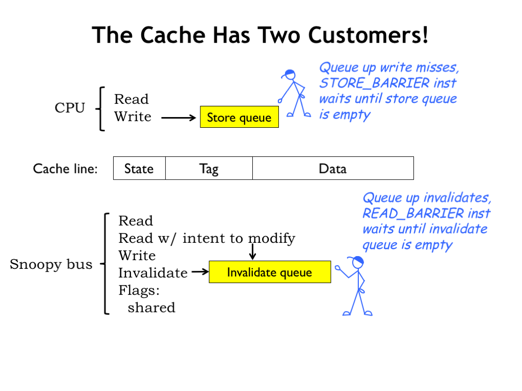
To support cache coherence, the cache hardware has to be modified to support two request streams: one from the CPU and one from the snoopy bus.
The CPU side includes a queue of store requests that were delayed by cache misses. This allows the CPU to proceed without having to wait for the cache refill operation to complete. Note that CPU read requests will need to check the store queue before they check the cache to ensure the most-recent value is supplied to the CPU. Usually there’s a STORE_BARRIER instruction that stalls the CPU until the store queue is empty, guaranteeing that all processors have seen the effect of the writes before execution resumes.
On the snoopy-bus side, the cache has to snoop on the transactions from other caches, invalidating or supplying cache line data as appropriate, and then updating the local cache line state. If the cache is busy with, say, a refill operation, INVALIDATE requests may be queued until they can be processed. Usually there’s a READ_BARRIER instruction that stalls the CPU until the invalidate queue is empty, guaranteeing that updates from other processors have been applied to the local cache state before execution resumes.
Note that the “read with intent to modify” transaction shown here is just protocol shorthand for a READ immediately followed by an INVALIDATE, indicating that the requester will be changing the contents of the cache line.
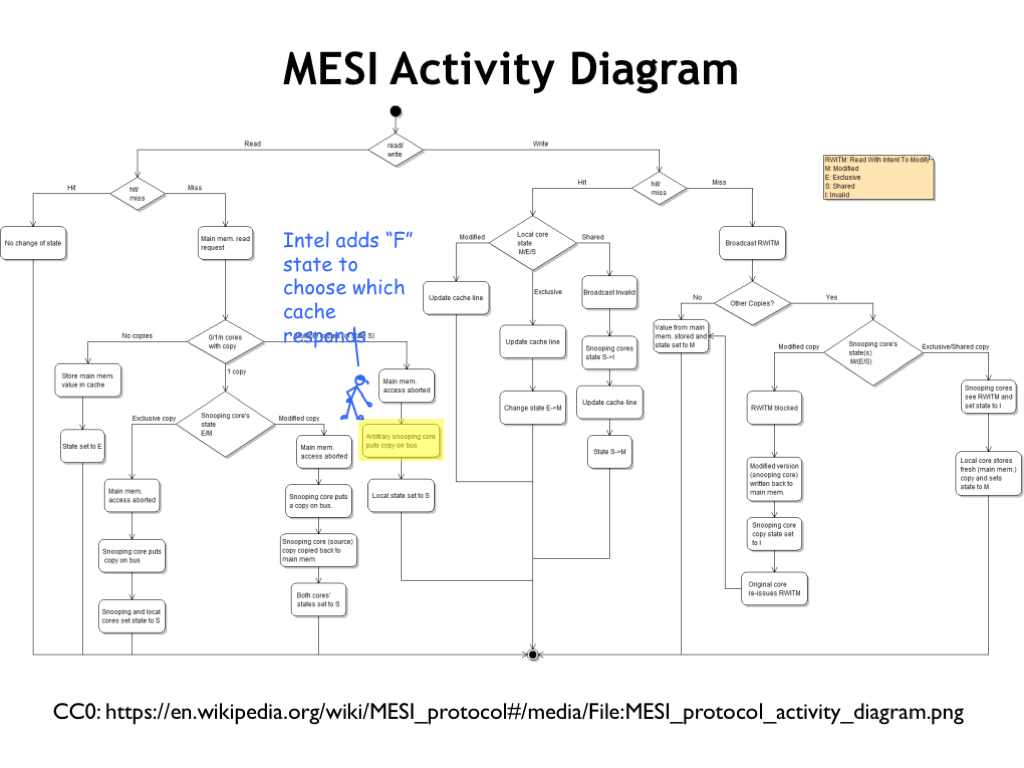
How do the CPU and snoopy-bus requests affect the cache state? Here in micro type is a flow chart showing what happens when. If you’re interested, try following the actions required to complete various transactions.
Intel, in its wisdom, adds a fifth “F” state, used to determine which cache will respond to read request when the requested cache line is shared by multiple caches — basically it selects which of the SHARED cache lines gets to be the responder.
But this is a bit abstract. Let’s try the MESI cache coherence protocol on our earlier example!
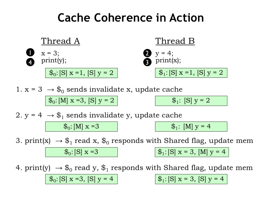
Here are our two threads and their local cache states indicating that values of locations X and Y are shared by both caches. Let’s see what happens when the operations happen in the order (1 through 4) shown here. You can check what happens when the transactions are in a different order or happen concurrently.
First, Thread A changes X to 3. Since this location is marked as SHARED [S] in the local cache, the cache for core 0 (\\(_0) issues an INVALIDATE transaction for location X to the other caches, giving it exclusive access to location X, which it changes to have the value 3. At the end of this step, the cache for core 1 (\\)_1) no longer has a copy of the value for location X.
In step 2, Thread B changes Y to 4. Since this location is marked as SHARED in the local cache, cache 1 issues an INVALIDATE transaction for location Y to the other caches, giving it exclusive access to location Y, which it changes to have the value 4.
In step 3, execution continues in Thread B, which needs the value of location X. That’s a cache miss, so it issues a read request on the snoopy bus, and cache 0 responds with its updated value, and both caches mark the location X as SHARED. Main memory, which is also watching the snoopy bus, also updates its copy of the X value.
Finally, in step 4, Thread A needs the value for Y, which results in a similar transaction on the snoopy bus.
Note the outcome corresponds exactly to that produced by the same execution sequence on a timeshared core since the coherence protocol guarantees that no cache has an out-of-date copy of a shared memory location. And both caches agree on the ending values for the shared variables X and Y.
If you try other execution orders, you’ll see that sequential consistency and shared memory semantics are maintained in each case. The cache coherency protocol has done its job!
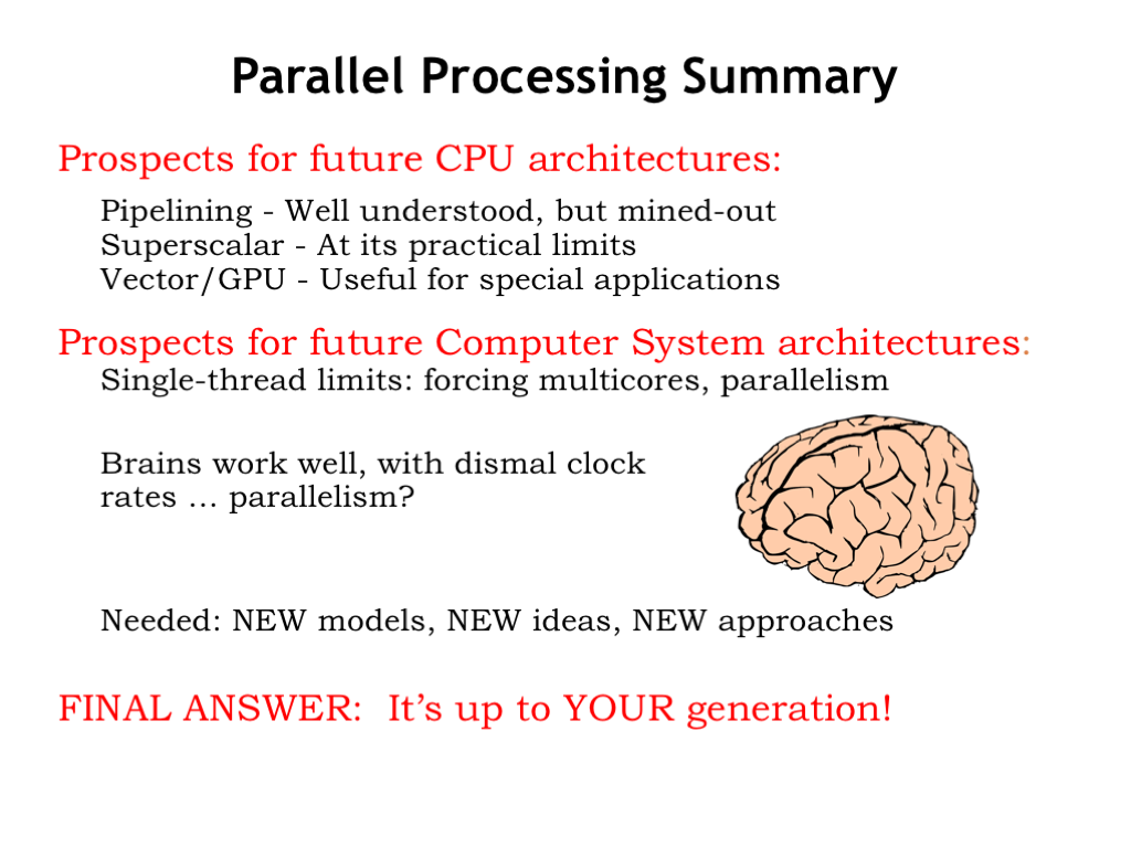
Let’s summarize our discussion of parallel processing.
At the moment, it seems that the architecture of a single core has reached a stable point. At least with the current ISAs, pipeline depths are unlikely to increase and out-of-order, superscalar instruction execution has reached the point of diminishing performance returns. So it seems unlikely there will be dramatic performance improvements due to architectural changes inside the CPU core. GPU architectures continue to evolve as they adapt to new uses in specific application areas, but they are unlikely to impact general-purpose computing.
At the system level, the trend is toward increasing the number of cores and figuring out how to best exploit parallelism with new algorithms.
Looking further ahead, notice that the brain is able to accomplish remarkable results using fairly slow mechanisms (it takes ~.01 seconds to get a message to the brain and synapses fire somewhere between 0.3 to 1.8 times per second). Is it massive parallelism that gives the brain its “computational” power? Or is it that the brain uses a different computation model, e.g., neural nets, to decide upon new actions given new inputs? At least for applications involving cognition there are new architectural and technology frontiers to explore. You have some interesting challenges ahead if you get interested in the future of parallel processing!


