Introduction To MATLAB Programming

Truth Statements and Logical Indexing

The Mandelbrot Set is the set of points \(z\in\mathbb{C}\) for which the sequence

\begin{equation} z_0=0,\quad z_{n+1}=(z_n)^2+z \label{eq:mandelbrot} \end{equation}

remains bounded as \(n\rightarrow\infty\). Color can be added for the unbounded elements by specifying how “fast” they diverge, for example, how many iterations it takes to reach some large absolute value. (Since once \(|x_n|\) is large enough the sequence will be growing indefinitely.)

To decide on the color of a particular point on the screen \((x,y)\), we define a complex number \(z=x+i y\) and iterate according to the equation mentioned above.

Exercise 17. With three nested for loops, iterate over x=-1.5:.01:0.5 and y=-1:0.01:1. For each point, iterate, say, 100 times and break if abs(z_n) is ever too large, say larger than 10. There’s no need to keep the sequence of \(z\)’s, but be sure not to overwrite the \(z\) variable that comes from \(x+iy\). If the the sequence grew to be large, leave white, otherwise place a black dot at (the original) \((x,y)\).

The result should look like this:

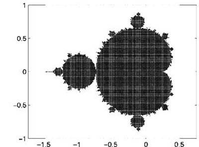
Graphing the Mandelbrot set.

Notice that it takes quite a long time to run, especially if you modify the code to give you a plot with better resolution. To fix this we want to use matrix-at-once calculation. We can create matrices X and Y using meshgrid:

x=-1.5:.1:1;
y=-1.5:.1:1.5;
[X,Y]=meshgrid(x,y);

Each element in these matrices holds the appropriate x- or y-value for that position in the matrix. We can now calculate the iterations very simply:

Z=X+1i*Y;   % use 1i since you can overwrite i but 1i will always be sqrt(-1)
Zn=0*Z;     % Start with zeros everywhere
Zn=Zn.^2+Z; 

Now that we know how to iterate we need to figure out how to color the different points. Here’s where the name of this subsection comes in.

Just as we can perform point-wise arithmetic with a matrix \(A\), we can also perform point-wise comparative and logical operations. The comparative operators are: > (greater than), < (less than) == (equal to**), ~= (not equal to), >= (greater than or equal to) <= (less than or equal to), while the logical operators are: ~ (not), & (and), | (or). For more help on operators type help ops.

Letting A=magic(4), understand the following constructions:

• A>5
• A<=3 | A>=10
• A==10 | A==5
• A>5 & A<10
• ~(A>5 & A<10)

Given that x = [1 5 2 8 9 0 1] and y = [5 2 2 6 0 0 2], execute and explain the results of the following commands:

1. x > y
2. y < x
3. x == y
4. x <= y
5. y >= x
6. x | y
7. x & y
8. x & (~y)
9. (x > y) | (y < x)
10. (x > y) & (y < x)

Together with the functions any and all we can ask questions like “Is any/all element of A equal to 4?”, the functions look down the first “non-singleton” dimension by default, which means that they work as you expect for column and row vectors, but for matrices they only “reduce” the first dimension:

>> any(magic(4)==4)      % by default reduces the first dimension (rows):
ans =
     1     0     0     0
>> any(magic(4)==4,2)    % we can tell it to reduce a different one:
ans =
     0
     0
     0
     1
>> any(any(magic(4)==4)) % To reduce a matrix to a single number, we must apply
                         % the functions twice:
ans =
     1

In addition we can use a truth matrix to access elements of a matrix. If we have a matrix A and a truth matrix (a matrix found by comparative and logical operations) B of the same size as A, we may write A(B) and the result will be the list (not matrix!) of elements of A for which the corresponding elements of B are “true.” This is slightly confusing, so an example is useful:

>> A=magic(4);
>> B=A>10;
>> A(B)
ans =
     16
     11
     14
     15
     13
     12

Exercise 18. Explain the order of the numbers in the previous example.

In addition to getting the list of elements that correspond to some truth matrix, we can also use the truth matrix to change specific elements of a matrix:

>> A
A =
     16     2     3    13
      5    11    10     8
      9     7     6    12
      4    14    15     1
>> A>5
ans =
     1     0     0     1
     0     1     1     1
     1     1     1     1
     0     1     1     0
>> A(A>5)=0
A =
     0     2     3     0
     5     0     0     0
     0     0     0     0
     4     0     0     1

Exercise 19. The exercises here show the techniques of logical indexing. Given x = 1:10 and y = [3 1 5 6 8 2 9 4 7 0], execute and interpret the results of the following commands:

1(a)	(x > 3) & (x < 8)
1(b)	x(x > 5)
1(c)	y(x <= 4)
1(d)	x( (x < 2) | (x >= 8) )
1(e)	y( (x < 2) | (x >= 8) )
1(f)	x(y < 0)

Given x = [3 15 9 12 -1 0 -12 9 6 1], provide the command(s) that will

2(a)	… set the positive elements of x to zero.
2(b)	… set values of x that are multiples of 3 to 3 (rem will help here).
2(c)	… multiply the even elements of x by 5.
2(d)	… extract the values of x that are greater than 10 into a vector called y.
2(e)	… set the values in x that are less than the mean value of x to zero.
2(f)	… set the values in x that are above the mean to their difference from the mean.

Homework 8. Going back to the Mandelbrot set calculation, we can keep a matrix that informs us of the step at which each element has become too large. Let’s call it Iter and agree that a zero value corresponds to “not too large yet” and a non-zero value will be the iteration number at which the element has become big (absolute value greater than 10). At each step we update only these elements of Zn that are still small (those that correspond to ~Iter being true), then find out which are the new big elements (abs(Zn)>10 and ~Iter) and set the corresponding values of Iter to the iteration number (from the for loop). Notice that using ~ on a matrix of numbers returns true for the elements that are zero and false for those that are not zero. After 100 iterations you need to plot the results. Since for the locations that did not converge we have the number of iterations it needs to reach size 10, we can make a nicer plot than the black-and-white plot from before. For this we can use:

p=pcolor(X,Y,Iter);
set(p,'edgecolor','none')
axis equal

We only need to plot once, after all the iterations have happened. Notice how much faster this is than the nested loops from before. Your result should look like this:

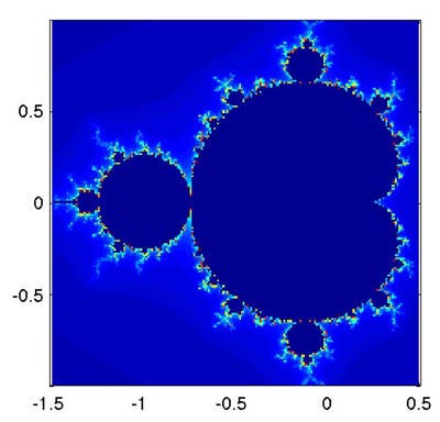
Graphing the Mandelbrot set with logical indexing.

Some ideas for “extra credit”:

• Try zooming into places of interest; see how the fractal is “self similar”?
• Change the number of iterations and see how things change.

**Make sure you understand the difference between = and ==; they mean entirely different things, and writing one instead of the other will most likely result in a strange error.