18.S997 | Fall 2011 | Undergraduate

Introduction To MATLAB Programming

Basic Plotting

Screenshot of plot commands and resultant red circle and black Lissajous curves.
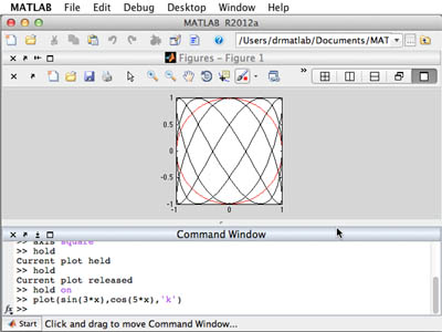
MATLAB can graph both functions and non-functions, as demonstrated by the circle and Lissajous curves.

In the previous unit, plotting was introduced with Newton’s method, but it is worthwhile to further explore the capabilities of plotting in MATLAB®. Preliminary exercises will encourage you to discover how to stylize your plots as well as plot multiple functions with the same plot command. To do this, you will be asked to plot different basins of attraction, sets of points that converge to a given root, for Newton’s method. We will generalize Newton’s method to higher dimensions by writing the function as a vector and finding the Jacobian matrix, which represents the linear approximation of the function. To visualize the basin of attraction, we will color a grid of points according to each point’s resultant root after iterating with Newton’s method.

The video below demonstrates, step-by-step, how to work with MATLAB in relevance to the topics covered in this unit.

Back to Newton’s method: It turns out that the end result (the point to which the method converges, if any) is strongly dependent on the initial guess. Furthermore, the dependence on the first guess can be rather surprising. The set of points that converge to a given root is called the basin of attraction of that root (for the iteration under discussion). I would like us to visualize the basins of attraction by coloring each starting point with a color that corresponds to the root it converges to. The different basins will thus be given different colors.

With MATLAB® we can easily visualize which solution is chosen as a function of the initial guess. While this can be done for 1D, we will do it for 2D and learn how to do some simple linear algebra at the same time.

Generalizing Newton’s method for higher dimensions is actually quite straightforward: Instead of one function \(f\), we have many, written as a vector \(\vec f\), and instead of one independent variable (\(x\)) we have many, again, written as a vector, \(\vec x\). Thus we are looking for the vector \(x\) for which:

\begin{equation} \label{eq:4} \vec f(\vec x)=\vec 0 \end{equation}

The update rule is slightly different since derivatives are more complicated in higher dimensions:

\begin{equation} \label{eq:newtons:multi:d} \vec x_{n+1}=\vec x_n- (J\vec f)^{-1} \vec f(\vec x_n). \end{equation}

Here \(Jf\) is the Jacobian matrix of \(\vec f\), that is a matrix whose term in the \(i-\)th row and \(j-\)th column is

\begin{equation} \label{eq:5} (J\vec f)_{ij}=\frac{\partial f_i}{\partial x_j}. \end{equation}

Notice that the Jacobian depends on \(\vec x\) and thus needs to be re-evaluated at every step (just like the derivative in one-dimensional Newton’s method). The two parts in the right-most term of (2) are multiplied together in the linear algebra sense of the word. The power \(-1\) is matrix inverse (and not multiplicative inverse) and thus another way of writing the update rule is

\begin{equation} \label{eq:6} (J\vec f) \delta\vec x_n= (J\vec f) (\vec x_{n+1}-\vec x_n)=-\vec f(\vec x_n). \end{equation}

This formulation is a much better way of understanding Newton’s method, as it exposes what is going on: The approximation is updated so that if the linear approximation to \(\vec f\) (given by the Jacobian matrix) were exact, the approximation would equal the exact root in one step.

How to implement? First we need a specific function: \(\vec f([x,y]^t)=[x^3-y,y^3-x]^t\) and thus the Jacobian matrix is \((\begin{smallmatrix} 3x^2 & -1 \\ -1& 3y^2 \end{smallmatrix})\). In MATLAB we want to have one variable, say \(X\), be a column vector that holds both \(x\) and \(y\). The code for a simple Newton method for \(f\) would be:

X=[1;2];   % the starting point. Notice the use of semicolon to define a column vector
for j=1:10 

Exercise 11. Multi-dimensional Newton’s method

  • What are the 3 roots of \(\vec f\) in the code above? (think of them as r1, r2, r3.)

  • Implement the program above and play around with the starting point to get several different answers. If you get a warning about singular matrices, don’t worry about it.

  • Find the Jacobian matrix, \(J\vec g\), of: 

    \begin{equation*} \vec g(\vec x)= \begin{pmatrix} \sin(x_1+2x_2^2)-x_2\\ x_1^2x_2-x_1 \end{pmatrix} \end{equation*}

  • The function \(g\) has many roots; modify the Newton solver to find some them by manually starting at different places.

  • Are you iterating enough times? Check that the results you get are a good enough root, and if they are not, change the number of iterations so that they are.

Now here’s the run-up to the next project: We want to plot the “basin of attraction” of each of the three zeros (what are they?) of the function \(\vec f\) (not \(\vec g\)). This will be your first project, but first we need to discuss how to plot the result. For an initial point \(X_0\) we can run the Newton code and after several iterations (10 in the example above) it will arrive near (in most cases) one of three roots, say \(r_1, r_2, r_3\). To visualize the basin of attraction, we go over a grid of points \(X_0\) and color them according to the to the specific zero the Newton’s method algorithm ends up being close to after starting from \(X_0\). If the algorithm is not close to any of them, we put a fourth color. While it is true that normally we do not know what the zeros are, but this is also interesting in the case that we do know what they are, so we are using the a priori information about the location of the roots in order to visualize the basin of attraction.

To do this we need if-else-end statements:

if norm(X-r1)<1e-8 % if the distance between X and r1 is less than 10^-8
     c='r';        % use the color red
elseif norm(X-r2)<1e-8
     c='b';        % use the color blue
elseif norm(X-r3)<1e-8
     c='g';        % use the color green
else               % if not close to any of the roots
     c='k';        % use the color black
end
plot(x,y,'.','color',c); % plot a point at X_0, (not the final point X!)
                         % with the color c

Project 1. Place the Newton code, and the if-then-else code above inside two nested for loops, looping over \(x-\) values and \(y-\) values from -2 to 2 (perhaps with a small step-size of 0.1 or 0.01). For each iteration set the starting point to [x,y]’ before the Newton’s Method part, and then plot the color point corresponding to the location of the resulting zero. So that the subsequent plot commands do not erase the previous ones, put:

clf % clear the current Figure
hold on % make sure subsequent plots do not erase the previous ones.

before the for loops. Thus the pseudo-code for this construction is:

initialize figure
for x values
     for y values
          let X0=(x,y) be the starting point for Newton's method
          find the color corresponding to the final point of iteration X
          plot point X0 with correct color
     end loop y
end loop x

If this is your first programming project, you might get frustrated at how difficult it seems to get everything in place. There’s no way around it. Read you own code carefully. Give good names to your variables. Try to explain the code to someone else.

That said, there are several hints I can give:

Hint 1. If MATLAB is stuck, use Ctrl C to abort from a long calculation or to reset the command line.
Hint 2. If MATLAB is spewing out too much onto the screen and you cannot see what you want to see, add semi-colons (;) to the end of the “offending” lines to prevent MATLAB from doing that.
Hint 3. If all the points seem to be plotted at the roots rather than at the original points, you are probably using \(X\) to do the plotting rather than the original point (x,y) from the loop.
Hint 4. If you are getting warnings from MATLAB that your “Matrix is close to singular or badly scaled” don’t worry about it too much. It means that your algorithm has passed through a point where the Jacobian matrix is singular. The result from that point is unreliable, but there should be (relatively) few of these points, and so the overall picture will be preserved.
Hint 5. If you always only have one point on your plot, you are probably not holding the plot properly. The two lines of code under the description of the project should be before the for loops (and not anywhere else).
Hint 6. What is the solution supposed to look like? My result can be seen in Fig. 1. Increasing the number of iterations should make the black regions (places that have not converged) smaller.

Colorful graphic with symmetry around a center point.

Figure 1. Basin of attraction for \(f([x,y]^t)=(x^3-y,y^3-x)^t\).

  • What do 1:10, 1:2:10 100:-25:0 do? Think, then check.

  • Let x = [2 5 1 6]. What will x(3), x([1 2]), x([1:end]), x(end:-1:1), x(:), x([1 1 1 1]) do? Think, guess, discuss with a friend, and finally, verify.

  • When creating a matrix, a space or a comma (,) are the separator between columns, while a semicolon (;) separate between rows. Figure out how to create the following matrices: \(\begin{pmatrix} 1& 2& 3\\ 4&5&6 \end{pmatrix}\), \(\begin{pmatrix} 1& 0 &1 \\ 0& 1& 0 \end{pmatrix}\)

  • You can nest matrix construction so that [ 6 (1:5) 7 ] makes sense (what does it result in?) Similarly you can create a matrix by stacking column vectors next to each other (using a space or a comma) or row vectors on top of each other (using a semicolon). Create the following matrix using a relatively short line of code:\begin{equation} \begin{pmatrix} 1 &2&3&4&5&6&7&8&9&10\\ 1&4&9&16&25&36&49&64&81&100\\ 2&4&8&16&32&64&128&256&512&1024 \end{pmatrix} \end{equation}

    Can you now easily make the first list go up to 100 (and the others follow suit)? If not, solve the problem again so that you can do it.

The plot command plots a list of points given as two vectors, \(X\) and \(Y\) of their x- and y- coordinates, respectively. The default behaviour is that no mark is placed on the points, and the points are joined by a straight line. So if we want to plot a parabola \(y=x^2\) for \(x\in[-1,1]\) we can write:

x=-1:.1:1;
y=x.^2;
plot(x,y)

Graph of an upward-facing parabola in blue.

Graphing a simple function, y=x^2.

We could make that line green by adding a third input:

x=-1:.1:1;
y=x.^2;
plot(x,y,'g.')

Graph of an upward-facing parabola with discontinuous green line markers.

Stylizing the graphs with colors and line markers.

The resulting plot need not be a function in the mathematical sense of the word:

t=-1:.01:2*pi;
x=sin(5*t);
y=cos(3*t);
plot(x,y,'r')

Graph of a Lissajous figure in red.

Graphing a non-function in MATLAB®.

Exercise 10. Read the helpfile on plot by typing help plot and figure out how to do the following:

  • Plot only the points and not the lines
  • Plot the parabola sideways (the result is not a function)
  • Plot using a red, dashed line and stars at each point
  • Make the plot with less points so that you can see that the lines between the points are straight
  • Plot the function \(\sin x\) vs. \(x\), for \(x\in [0,6\pi]\)
  • Figure out how to plot two functions with the same plot command, and plot \(\sin x\) and \(\cos x\) vs. \(x\).

Course Info

Instructor
Departments
As Taught In
Fall 2011
Learning Resource Types
Problem Sets
Lecture Videos
Online Textbook
Programming Assignments with Examples