Fractals and Chaos

$Graph of 100 iterations of the Mandelbrot fractal.$
Generating fractals is a comprehensive way to utilize MATLAB®’s programming loops and logical expressions.

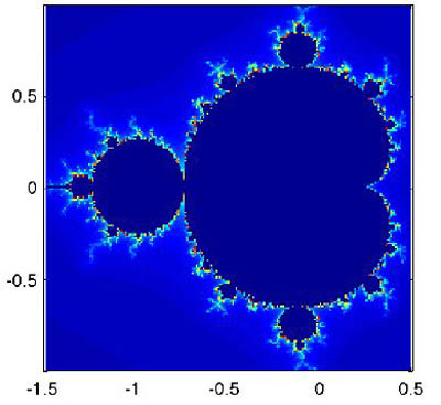
A fractal is a geometric figure that can be subdivided into parts that are mathematically similar to the whole. You will be asked to plot the Mandelbrot fractal, and effectively practice constructing while loops, which terminate based on a known and specified condition. You will also learn how to use commands that help you terminate the loop prematurely and otherwise modify the execution of the loop.

In this unit, you will also use comparative and logical operations to evaluate expressions and create a truth matrix composed of zeroes and ones. The truth matrix will be useful for logical indexing, which can be used in situations that require that certain elements of a list be separated from the rest of the elements based on a certain characteristic.

Homework 4. For $r$ varying between 0 and 4, find out the possible “limit cycles"^§ of the iterative map:

\begin{equation} x_{n+1}=r x_n(1-x), \qquad x_0= 0.5 \text{(or anything else that is not $0$ nor $1$)} \end{equation}

This converges to a single value for some values of $r$ but for others results in an “orbit”, which can be very long. For every $0<r<4$, “find” this orbit and plot the orbits together.

Use the “matrix-at-a-time” notation we learned in the last iteration example:

Start with a vector of $r-$values, and a vector of $x-$values (both row vectors and the same size).
Perform many (how many?) iterations on the whole vector of $x-$values, so that each place in the vector is updated according to its appropriate $r$.
Plot the resulting $x$-values vs. the $r$ values.
Continue the iteration and plot several more iterations (how many?).
Observe the nice pattern that arises, and explore its self-similarity properties.

Hint 1: (Am I getting the right answer?) The result should look something like this:

Plot of many iterations of a function that branches to the right.

Graphing an iterative function.

Hint 2: (Code takes forever) If your code is running very slowly, you should consider updating all the orbits (one for each $r$ value) at once. This implies holding a vector that corresponds to the $r$ values you are considering, and a vector corresponding to the various orbits, and with one line of code you can update all the values in the orbit. Do this in a loop to find “late” elements of the orbit.

Hint 3: (Getting a similar plot, but not quite) You should only plot the late elements, so perhaps iterate without plotting for some time (maybe 1000 iterations?) and then plot successive elements of the orbit (say 100?).

Hint 4: (I don’t have so many points in my plot) Be sure to use hold on so that each plot doesn’t erase the previous ones.

More ideas:

Find how to make the plot have small dots as markers.
Can you allow the user to “zoom in” on your plot? Once asked to see a region smaller than $(0, 4)\times(0, 1)$ you should probably increase the “density” of your $r$ measurements, and confine the plotting of the points so that only the requested $x$’s are plotted.

^§a limit cycle is an orbit of an iterative map that the dynamics of the problem converges to, regardless of the initial condition.

The for loop is a very useful tool for doing things over and over again for a certain number of times already known in advance. There are two possibilities that we would like to consider:

What if we do not know in advance how many iterations we will need?
What if we would like to stop a loop before it is due to end?

An example for the first kind would be a Newton iteration that should run until the value of $f(x)$ is “small” enough, for example $10^{-12}$. Before actually performing the iterations we do not know how many steps it will take, so a for loop is not exactly the right type of loop. We could get around this limitation if we introduce a maximum number of allowed iterations and then use the (as-of-yet unknown) mechanism for terminating a loop prematurely once we find a good enough approximate root.

A while loop tells MATLAB® to continue iterating as long as a certain condition (which you specify) is satisfied. The syntax is:

while <condition>
   <statements> end

MATLAB evaluates the <condition> and if it is true (or a non-zero number) it performs the <statements>, if not, it continues after the end. After each time it evaluates <statements> MATLAB goes back and evaluates <condition> again, etc. Note that <condition> does not get evaluated in the middle of evaluating <statements> but, rather, only before evaluating them. Here’s a simple way of adding two positive integers (very silly):

x=5;
y=6;
while y>0
    x=x+1;
    y=y-1;

Of course, this fails miserably if y is not a positive integer (doesn’t do anything, do you understand why?)

Exercise 16. Solve the following problems using a while loop:

Show the numbers from 1 to 10
Show the numbers from 10 to -10
_Find out how many divisors 28 has (_mod or rem will be useful here)
Find out if a number is prime
Use an external while and an internal for loop to find the first 100 prime numbers.
A perfect number is a number $n$ whose divisors (including 1 but excluding itself) add up to $n$ itself. For example, 6 is a perfect number. Check if a number is perfect.
Use two nested while loops to find the first 3 perfect numbers.

Homework 5. Consider the following sequence defined completely by the first element $S_1$^¶:

\begin{equation} S_{n+1}= \begin{cases} S_n/2 & \text{ if } S_n \text{ is even}\\ 3 S_n+1 & \text{ if } S_n \text{ is odd} \end{cases} \end{equation}

_A still_^|| open question in mathematics is whether all such sequences always arrive at 1 for large enough $n$ (the alternatives being that some sequences may rise indefinitely, or that there may be a closed orbit that does not include 1). Compute the number of iterations it takes to arrive at $1$ given a starting value $s$ using a while loop. Since we do not know how long it will take to arrive at 1 (though you can assume that it will happen eventually) we might want to construct this sequence using a while-loop. What starting number smaller than 10,000 has the longest trajectory? What’s the largest number on that trajectory?

^§This is the subject of the Collatz Conjecture.

^||Despite a recent “near” solution.

As you may recall, a while loop will evaluate all its statements without checking the condition. Similarly a for loop will run through all of its iterations. The break keyword tells MATLAB® to exit the loop immediately. It will only terminate one loop (in the case of nested loop, the innermost one it is in) and will normally be protected by an if statement (otherwise the loop is silly). Here is an example that computes the “trajectory” of 6 but stops if it finds a 17 in it:

s=6;             % initialize s to 6
while s~=1       % as long as s is not equal to 1 stay in the loop
     if s==17    % if s equals 17
          sprintf('Found 17 in the loop!!')
          break;
     end
     if mod(s,2) % the actual "brains" of the iteration
          s=s/2;
     else
          s=3*s+1;

The keyword continue is similar but different. It avoids the rest of the statements of the inner most loop, but continues in the loop (does not stop like break).

Here’s example code for a while loop that uses both break and continue to find the first 100 primes (not very efficiently, but it’s only an example):

n=1;
m=0;

while 1      % this means that unless we use "break", the loop will continue "forever"
     n=n+1;  % increase n
     flag=0; % reset flag
     for i=2:ceil(sqrt(n)) % no need to check numbers greater than the square-root of n
          if mod(n,i)==0   % means that i divides n exactly
               flag = 1    % to know that we found a divisor
               break;      % no need to remain in the for loop
          end
     end
     if flag
          continue % to avoid the next line. It could have also been done
                   % differently with an "if" statement, but this can be more elegant
     end
     sprintf('%d is prime!\n',n) % this is quite an interesting command...
                                 % take some time to learn about it
     m=m+1;      % increment primes count
     if m>=100   % if we have enough
          break; % stop looking for primes
     end
end

Homework 6. The keywords break and continue are not “needed’’ per se, but they can make the code more elegant and readable. Rewrite the above code for the first 100 primes without using neither continue nor break.

Homework 7. for loops and while loops are not inherently different:

The “input” of a for loop is a variable and a vector of values. Recreate the functionality of a for loop using a while loop.
The “input” of a while loop is the condition statement. Recreate the functionality of a while loop using a for loop. (Hint: when using the notation for i=1:n MATLAB does not actually create the vector 1:n. Internally it simply iterates over the values in that vector by incrementing i until it reaches n. This means that if you write for i=1:281474976710655 you’ll get a loop that, on its own, will “never” terminate. Explanation: 281474976710655 is the largest integer that MATLAB can represent internally. It is such a large number that even if every pass through the loop only takes 1 millisecond getting through the loop will take about 10000 years.)

The Mandelbrot Set is the set of points $z\in\mathbb{C}$ for which the sequence

\begin{equation} z_0=0,\quad z_{n+1}=(z_n)^2+z \label{eq:mandelbrot} \end{equation}

remains bounded as $n\rightarrow\infty$. Color can be added for the unbounded elements by specifying how “fast” they diverge, for example, how many iterations it takes to reach some large absolute value. (Since once $|x_n|$ is large enough the sequence will be growing indefinitely.)

To decide on the color of a particular point on the screen $(x,y)$, we define a complex number $z=x+i y$ and iterate according to the equation mentioned above.

Exercise 17. With three nested for loops, iterate over x=-1.5:.01:0.5 and y=-1:0.01:1. For each point, iterate, say, 100 times and break if abs(z_n) is ever too large, say larger than 10. There’s no need to keep the sequence of $z$’s, but be sure not to overwrite the $z$ variable that comes from $x+iy$. If the the sequence grew to be large, leave white, otherwise place a black dot at (the original) $(x,y)$.

The result should look like this:

$Graph of 100 iterations of the Mandelbrot fractal in gray.$

Graphing the Mandelbrot set.

Notice that it takes quite a long time to run, especially if you modify the code to give you a plot with better resolution. To fix this we want to use matrix-at-once calculation. We can create matrices X and Y using meshgrid:

x=-1.5:.1:1;
y=-1.5:.1:1.5;
[X,Y]=meshgrid(x,y);

Each element in these matrices holds the appropriate x- or y-value for that position in the matrix. We can now calculate the iterations very simply:

Z=X+1i*Y;   % use 1i since you can overwrite i but 1i will always be sqrt(-1)
Zn=0*Z;     % Start with zeros everywhere
Zn=Zn.^2+Z;

Now that we know how to iterate we need to figure out how to color the different points. Here’s where the name of this subsection comes in.

Just as we can perform point-wise arithmetic with a matrix $A$, we can also perform point-wise comparative and logical operations. The comparative operators are: > (greater than), < (less than) == (equal to**), ~= (not equal to), >= (greater than or equal to) <= (less than or equal to), while the logical operators are: ~ (not), & (and), | (or). For more help on operators type help ops.

Letting A=magic(4), understand the following constructions:

A>5
A<=3 | A>=10
A==10 | A==5
A>5 & A<10
~(A>5 & A<10)

Given that x = [1 5 2 8 9 0 1] and y = [5 2 2 6 0 0 2], execute and explain the results of the following commands:

x > y
y < x
x == y
x <= y
y >= x
x | y
x & y
x & (~y)
(x > y) | (y < x)
(x > y) & (y < x)

Together with the functions any and all we can ask questions like “Is any/all element of A equal to 4?”, the functions look down the first “non-singleton” dimension by default, which means that they work as you expect for column and row vectors, but for matrices they only “reduce” the first dimension:

>> any(magic(4)==4)      % by default reduces the first dimension (rows):
ans =
     1     0     0     0
>> any(magic(4)==4,2)    % we can tell it to reduce a different one:
ans =
     0
     0
     0
     1
>> any(any(magic(4)==4)) % To reduce a matrix to a single number, we must apply
                         % the functions twice:
ans =
     1

In addition we can use a truth matrix to access elements of a matrix. If we have a matrix A and a truth matrix (a matrix found by comparative and logical operations) B of the same size as A, we may write A(B) and the result will be the list (not matrix!) of elements of A for which the corresponding elements of B are “true.” This is slightly confusing, so an example is useful:

>> A=magic(4);
>> B=A>10;
>> A(B)
ans =
     16
     11
     14
     15
     13
     12

Exercise 18. Explain the order of the numbers in the previous example.

In addition to getting the list of elements that correspond to some truth matrix, we can also use the truth matrix to change specific elements of a matrix:

>> A
A =
     16     2     3    13
      5    11    10     8
      9     7     6    12
      4    14    15     1
>> A>5
ans =
     1     0     0     1
     0     1     1     1
     1     1     1     1
     0     1     1     0
>> A(A>5)=0
A =
     0     2     3     0
     5     0     0     0
     0     0     0     0
     4     0     0     1

Exercise 19. The exercises here show the techniques of logical indexing. Given x = 1:10 and y = [3 1 5 6 8 2 9 4 7 0], execute and interpret the results of the following commands:

1(a)	(x > 3) & (x < 8)
1(b)	x(x > 5)
1(c)	y(x <= 4)
1(d)	x( (x < 2) \| (x >= 8) )
1(e)	y( (x < 2) \| (x >= 8) )
1(f)	x(y < 0)

Given x = [3 15 9 12 -1 0 -12 9 6 1], provide the command(s) that will

2(a)	… set the positive elements of x to zero.
2(b)	… set values of x that are multiples of 3 to 3 (rem will help here).
2(c)	… multiply the even elements of x by 5.
2(d)	… extract the values of x that are greater than 10 into a vector called y.
2(e)	… set the values in x that are less than the mean value of x to zero.
2(f)	… set the values in x that are above the mean to their difference from the mean.

Homework 8. Going back to the Mandelbrot set calculation, we can keep a matrix that informs us of the step at which each element has become too large. Let’s call it Iter and agree that a zero value corresponds to “not too large yet” and a non-zero value will be the iteration number at which the element has become big (absolute value greater than 10). At each step we update only these elements of Zn that are still small (those that correspond to ~Iter being true), then find out which are the new big elements (abs(Zn)>10 and ~Iter) and set the corresponding values of Iter to the iteration number (from the for loop). Notice that using ~ on a matrix of numbers returns true for the elements that are zero and false for those that are not zero. After 100 iterations you need to plot the results. Since for the locations that did not converge we have the number of iterations it needs to reach size 10, we can make a nicer plot than the black-and-white plot from before. For this we can use:

p=pcolor(X,Y,Iter);
set(p,'edgecolor','none')
axis equal

We only need to plot once, after all the iterations have happened. Notice how much faster this is than the nested loops from before. Your result should look like this:

$Graph of 100 iterations of the Mandelbrot fractal.$

Graphing the Mandelbrot set with logical indexing.

Some ideas for “extra credit”:

Try zooming into places of interest; see how the fractal is “self similar”?
Change the number of iterations and see how things change.

**Make sure you understand the difference between = and ==; they mean entirely different things, and writing one instead of the other will most likely result in a strange error.

Browse Course Material

Course Info

Instructor

Departments

As Taught In

Level

Topics

Learning Resource Types

Introduction To MATLAB Programming