
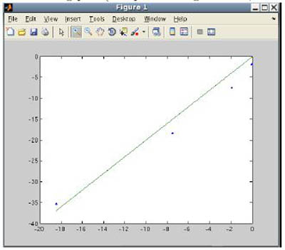
MATLAB can calculate roots through Newton’s method, and verification of convergence is graphed.
Now that you are familiar with MATLAB® and its basic functionalities, you will learn how to use MATLAB to find the roots of equations, and specifically, nonlinear equations. We will walk through using Newton’s method for this process, and step through multiple iterations of Newton’s method in order to arrive at a final solution.
Because Newton’s method is an iterative process, you will also learn how to construct two types of logical loops: for loops and while loops. These loops will be useful tools not just for the purpose of using Newton’s method, but also for future use in writing code that can handle more complicated operations. In addition to learning how to construct loops, you will be introduced to plotting in MATLAB and saving code in a file for future or frequent use.
The secant method is presented as an alternative to Newton’s method, and you will be asked to use MATLAB in comparing the convergence of solutions—essentially, the speed at which they can approximate a solution—from these respective methods. When completing this portion of the unit, you will find the need to store multiple values for comparison, and this offers the opportunity to make use of lists and sublists through sub-indexing. Since discrepancies in syntax are important when it comes to using and operating on lists and matrices in MATLAB, you will be asked to evaluate a variety of expressions that help you understand these differences.
Related Videos
The videos below demonstrate, step-by-step, how to work with MATLAB in relation to the topics covered in this unit.
- Lecture 3: Using Files
This video includes material supplementary to The Secant Method. - Lecture 6: Debugging
This video includes material supplementary to The Secant Method.


